如何解释「卷积神经网络」?

神经网络由具有权重和偏差的神经元组成。通过在训练过程中调整这些权重和偏差,以提出良好的学习模型。每个神经元接收一组输入,以某种方式处理它,然后输出一个值。如果构建一个具有多层的神经网络,则将其称为深度神经网络。处理这些深度神经网络的人工智能学分支被称为深度学习。

普通神经网络的主要缺点是其忽略了输入数据的结构。在将数据馈送到神经网络之前,所有数据都将转换为一维数组。这适用于常规数据,但在处理图像时会遇到困难。
考虑到灰度图像是2D结构,像素的空间排列有很多隐藏信息。若忽略这些信息,则将失去许多潜在的模式。这就是卷积神经网络(CNN)被引入图像处理的原因。CNN在处理图像时会考虑图像的2D结构。
CNN也是由具有权重和偏差的神经元组成。这些神经元接收输入的数据并处理,然后输出信息。神经网络的目标是将输入层中的原始图像数据转到输出层中的正确类中。普通神经网络和CNN之间的区别在于使用的层类型以及处理输入数据的方式。假设CNN的输入是图像,这允许其提取特定于图像的属性。这使得CNN在处理图像方面更有效率。那么,CNN是如何构建的?


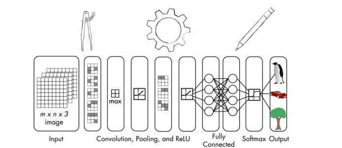
CNN的体系结构
当使用普通神经网络时,需要将输入数据转换为单个向量。该向量作为神经网络的输入,然后向量穿过神经网络的各层。在这些层中,每个神经元都与前一层中的所有神经元相连接。值得注意的是,同层的神经元互不连接。它们仅与相邻层的神经元相连。网络中的最后一层是输出层,它代表最终输出。
若将这种结构用于图像处理,它将很快变得难以管理。例如,一个由256x256RGB图像组成的图像数据集。由于这是3维图像,因此将有256 * 256 * 3 = 196,608个权重。请意,这仅适用于单个神经元!每层都有多个神经元,因此权重的数量迅速增加。这意味着在训练过程中,该模型将需要大量参数来调整权重。这就是该结构复杂和耗时的原因。将每个神经元连接到前一层中的每个神经元,称为完全连接,这显然不适用于图像处理。
CNN在处理数据时明确考虑图像的结构。CNN中的神经元按三维排列——宽度、高度和深度。当前层中的每个神经元都连接到前一层输出的小块。这就像在输入图像上叠加NxN过滤器一样。这与完全连接的层相反,完全连接层的每个神经元均与前一层的所有神经元相连。
由于单个过滤器无法捕获图像的所有细微差别,因此需要花费数倍的时间(假设M倍)确保捕获所有细节。这M个过滤器充当特征提取器。如果查看这些过滤器的输出,可以查看层的提取特征,如边缘、角等。这适用于CNN中的初始层。随着在神经网络层中的图像处理的进展,可看到后面的层将提取更高级别的特征。

CNN中的层类型
了解了CNN的架构,继续看看用于构建CNN各层的类型。CNN通常使用以下类型的层:
· 输入层:用于原始图像数据的输入。
· 卷积层:该层计算神经元与输入中各种切片之间的卷积。
快速了解图像卷积传送门:
http://web.pdx.edu/~jduh/courses/Archive/geog481w07/Students/Ludwig_ImageConvolution.pdf。
卷积层基本上计算权重和前一层输出的切片之间的点积。
· 激励层:此图层将激活函数应用于前一图层的输出。该函数类似于max(0,x)。需要向该层神经网络增加非线性映射,以便它可以很好地概括为任何类型的功能。
· 池化层:此层对前一层的输出进行采样,从而生成具有较小维度的结构。在网络中处理图像时,池化有助于只保留突出的部分。最大池是池化层最常用的,可在给定的KxK窗口中选择最大值。
· 全连接层:此图层计算最后一层的输出分。输出结果的大小为1x1xL,其中L是训练数据集中的类数。
从神经网络中的输入层到输出层时,输入图像将从像素值转换为最终的类得分。现已提出了许多不同的CNN架构,它是一个活跃的研究领域。模型的准确性和鲁棒性取决于许多因素- 层的类型、网络的深度、网络中各种类型的层的排列、为每层选择的功能和训练数据等。


构建基于感知器的线性回归量
接下来是有关如何用感知器构建线性回归模型。
本文将会使用TensorFlow。它是一种流行的深度学习软件包,广泛用于构建各种真实世界的系统中。在本节,我们将熟悉它的工作原理。在使用软件包前先安装它。
安装说明传送门:
https://http://www.tensorflow.org/get_started/os_setup。
确保它已安装后,创建一个新的python程序并导入以下包:
import numpy as np
import matplotlib.pyplot as plt
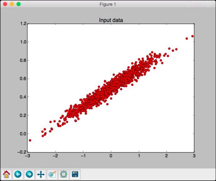
import tensorflow as tf使模型适应生成的数据点。定义要生成的数据点的数量:
# Define the number of points to generate
num_points = 1200
定义将用于生成数据的参数。使用线性模型:y =mx + c:
# Generate the data based on equation y = mx + c
data = []
m = 0.2
c = 0.5
for i in range(num_points):
    # Generate 'x'
    x = np.random.normal(0.0, 0.8)
生成的噪音使数据发生变化:
# Generate some noise
    noise = np.random.normal(0.0, 0.04)
使用以下等式计算y的值:
# Compute 'y'
    y = m*x + c + noise

    data.append([x, y])
完成迭代后,将数据分成输入和输出变量:
# Separate x and y
x_data = [d[0] for d in data]
y_data = [d[1] for d in data
绘制数据:
# Plot the generated data
plt.plot(x_data, y_data, 'ro')
plt.title('Input data')
plt.show()
为感知器生成权重和偏差。权重由统一的随机数生成器生成,并将偏差设置为零:
# Generate weights and biases
W = tf.Variable(tf.random_uniform([1], -1.0, 1.0))
b = tf.Variable(tf.zeros([1]))
使用TensorFlow变量定义等式:
# Define equation for 'y'
y = W * x_data + b
定义训练过程使用的损失函数。优化器将使损失函数的值尽可能地减小。
# Define how to compute the loss
loss = tf.reduce_mean(tf.square(y - y_data))
定义梯度下降优化器并指定损失函数:
# Define the gradient descent optimizer
optimizer = tf.train.GradientDescentOptimizer(0.5)
train = optimizer.minimize(loss)
所有变量都已到位,但尚未初始化。接下来:
# Initialize all the variables
init = tf.initialize_all_variables()
启动TensorFlow会话并使用初始化程序运行它:
# Start the tensorflow session and run it
sess = tf.Session()
sess.run(init)
开始训练:
# Start iterating
num_iterations = 10
for step in range(num_iterations):
    # Run the session
    sess.run(train)
打印训练进度。进行迭代时,损失参数将持续减少:
# Print the progress
print('\nITERATION', step+1)
print('W =', sess.run(W)[0])
print('b =', sess.run(b)[0])
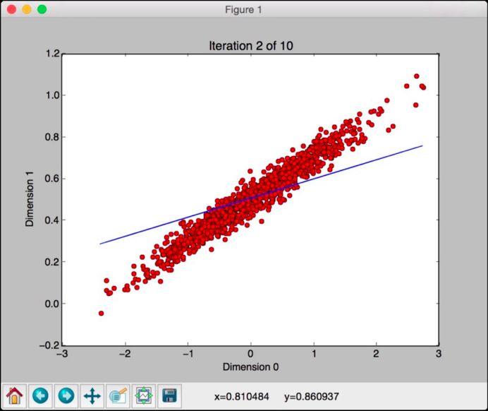
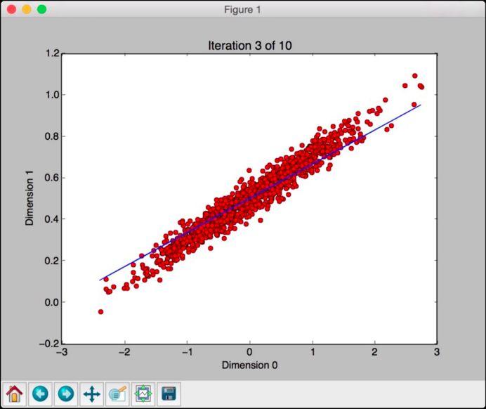
print('loss =', sess.run(loss))绘制生成的数据并在顶部覆盖预测的模型。该情况下,模型是一条线:
# Plot the input data
    plt.plot(x_data, y_data, 'ro')
    # Plot the predicted output line
    plt.plot(x_data, sess.run(W) * x_data + sess.run(b))
设置绘图的参数:
# Set plotting parameters
    plt.xlabel('Dimension 0')
    plt.ylabel('Dimension 1')
    plt.title('Iteration ' + str(step+1) + ' of ' + str(num_iterations))
    plt.show()
完整代码在linear_regression.py文件中给出。运行代码将看到以下屏幕截图显示输入数据:

如果关闭此窗口,将看到训练过程。第一次迭代看起来像这样:
可看到,线路完全偏离模型。关闭此窗口以转到下一个迭代:

这条线似乎更好,但它仍然偏离模型。关闭此窗口并继续迭代:

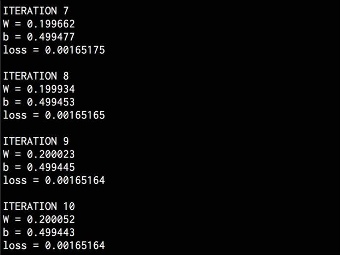
看起来这条线越来越接近真实的模型。如果继续像这样迭代,模型会变得更好。第八次迭代看起来如下:
该线与数据拟合的很好。将在终端上看到以下内容:
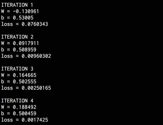

完成训练后,在终端上看到以下内容:

使用单层神经网络构建图像分类器
如何使用TensorFlow创建单层神经网络,并使用它来构建图像分类器?使用MNIST图像数据集来构建系统。它是包含手写的数字图像的数据集。其目标是构建一个能够正确识别每个图像中数字的分类器。

创建新的python程序并导入以下包:
import argparse
import tensorflow as tf
from tensorflow.examples.tutorials.mnist import input_data
定义一个解析输入参数的函数:
def build_arg_parser():
    parser = argparse.ArgumentParser(description='Build a classifier using
            \MNIST data')
    parser.add_argument('--input-dir', dest='input_dir', type=str,
            default='./mnist_data', help='Directory for storing data')
    return parser
定义main函数并解析输入参数:
if __name__ == '__main__':
    args = build_arg_parser().parse_args()
提取MNIST图像数据。one_hot标志指定将在标签中使用单热编码。这意味着如果有n个类,那么给定数据点的标签将是长度为n的数组。此数组中的每个元素都对应一个特定的类。要指定一个类,相应索引处的值将设置为1,其他所有值为0:
# Get the MNIST data
    mnist = input_data.read_data_sets(args.input_dir, one_hot=True)
数据库中的图像是28 x 28像素。需将其转换为单维数组以创建输入图层:
# The images are 28x28, so create the input layer
    # with 784 neurons (28x28=784)
    x = tf.placeholder(tf.float32, [None, 784])
创建具有权重和偏差的单层神经网络。数据库中有10个不同的数字。输入层中的神经元数量为784,输出层中的神经元数量为10:
# Create a layer with weights and biases. There are 10 distinct
    # digits, so the output layer should have 10 classes
    W = tf.Variable(tf.zeros([784, 10]))
    b = tf.Variable(tf.zeros([10]))
创建用于训练的等式:
# Create the equation for 'y' using y = W*x + b
    y = tf.matmul(x, W) + b
定义损失函数和梯度下降优化器:
# Define the entropy loss and the gradient descent optimizer
    y_loss = tf.placeholder(tf.float32, [None, 10])
    loss = tf.reduce_mean(tf.nn.softmax_cross_entropy_with_logits(y, y_loss))
    optimizer = tf.train.GradientDescentOptimizer(0.5).minimize(loss)
初始化所有变量:
# Initialize all the variables
    init = tf.initialize_all_variables()
创建TensorFlow会话并运行:
# Create a session
    session = tf.Session()
    session.run(init)
开始训练过程。使用当前批次运行优化器的批次进行训练,然后继续下一批次进行下一次迭代。每次迭代的第一步是获取下一批要训练的图像:
# Start training
    num_iterations = 1200
    batch_size = 90
    for _ in range(num_iterations):
        # Get the next batch of images
        x_batch, y_batch = mnist.train.next_batch(batch_size)
在这批图像上运行优化器:
# Train on this batch of images
        session.run(optimizer, feed_dict = {x: x_batch, y_loss: y_batch})
训练过程结束后,使用测试数据集计算准确度:
# Compute the accuracy using test data
    predicted = tf.equal(tf.argmax(y, 1), tf.argmax(y_loss, 1))
    accuracy = tf.reduce_mean(tf.cast(predicted, tf.float32))
    print('\nAccuracy =', session.run(accuracy, feed_dict = {
            x: mnist.test.images,
            y_loss: mnist.test.labels}))
完整代码在single_layer.py文件中给出。如果运行代码,它会将数据下载到当前文件夹中名为mnist_data的文件夹中。这是默认选项。如果要更改它,可以使用输入参数执行此操作。运行代码后,将在终端上获得以下输出:
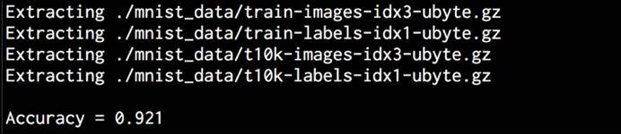

正如终端上打印所示,模型的准确率为92.1%。

使用卷积神经网络构建图像分类器
上一节中的图像分类器表现不佳。获得92.1%的MNIST数据集相对容易。如何使用卷积神经网络(CNN)来实现更高的精度呢?下面将使用相同的数据集构建图像分类器,但使用CNN而不是单层神经网络。
创建一个新的python程序并导入以下包:
import argparse
import tensorflow as tf
from tensorflow.examples.tutorials.mnist import input_data
定义一个解析输入参数的函数:
def build_arg_parser():
    parser = argparse.ArgumentParser(description='Build a CNN classifier \
            using MNIST data')
    parser.add_argument('--input-dir', dest='input_dir', type=str,
            default='./mnist_data', help='Directory for storing data')
    return parser
定义一个函数来为每个层中的权重创建值:
def get_weights(shape):
    data = tf.truncated_normal(shape, stddev=0.1)
    return tf.Variable(data)
定义一个函数来为每个层中的偏差创建值:
def get_biases(shape):
    data = tf.constant(0.1, shape=shape)
    return tf.Variable(data)
定义一个函数以根据输入形状创建图层:
def create_layer(shape):
    # Get the weights and biases
    W = get_weights(shape)
    b = get_biases([shape[-1]])

    return W, b
定义执行2D卷积功能的函数:
def convolution_2d(x, W):
    return tf.nn.conv2d(x, W, strides=[1, 1, 1, 1],
            padding='SAME')
定义一个函数来执行2x2最大池操作:
def max_pooling(x):
    return tf.nn.max_pool(x, ksize=[1, 2, 2, 1],
            strides=[1, 2, 2, 1], padding='SAME')
定义main函数并解析输入参数:
if __name__ == '__main__':
    args = build_arg_parser().parse_args()
提取MNIST图像数据:
# Get the MNIST data
    mnist = input_data.read_data_sets(args.input_dir, one_hot=True)
使用784个神经元创建输入层:
# The images are 28x28, so create the input layer
    # with 784 neurons (28x28=784)
    x = tf.placeholder(tf.float32, [None, 784])
接下来是利用图像2D结构的CNN。为4D张量,其中第二维和第三维指定图像尺寸:
# Reshape 'x' into a 4D tensor
    x_image = tf.reshape(x, [-1, 28, 28, 1])
创建第一个卷积层,为图像中的每个5x5切片提取32个要素:
# Define the first convolutional layer
    W_conv1, b_conv1 = create_layer([5, 5, 1, 32])
用前一步骤中计算的权重张量卷积图像,然后为其添加偏置张量。然后,需要将整流线性单元(ReLU)函数应用于输出:
# Convolve the image with weight tensor, add the
    # bias, and then apply the ReLU function
    h_conv1 = tf.nn.relu(convolution_2d(x_image, W_conv1) + b_conv1)
将2x2 最大池运算符应用于上一步的输出:
# Apply the max pooling operator
    h_pool1 = max_pooling(h_conv1)
创建第二个卷积层计算每个5x5切片上的64个要素:
# Define the second convolutional layer
    W_conv2, b_conv2 = create_layer([5, 5, 32, 64])
使用上一步中计算的权重张量卷积前一层的输出,然后添加偏差张量。然后,需要将整流线性单元(ReLU)函数应用于输出:
# Convolve the output of previous layer with the
    # weight tensor, add the bias, and then apply
    # the ReLU function
    h_conv2 = tf.nn.relu(convolution_2d(h_pool1, W_conv2) + b_conv2)
将2x2最大池运算符应用于上一步的输出:
# Apply the max pooling operator
    h_pool2 = max_pooling(h_conv2)
图像尺寸减少到了7x7。创建一个包含1024个神经元的完全连接层:
# Define the fully connected layer
    W_fc1, b_fc1 = create_layer([7 * 7 * 64, 1024])
重塑上一层的输出:
# Reshape the output of the previous layer
    h_pool2_flat = tf.reshape(h_pool2, [-1, 7*7*64])
将前一层的输出与完全连接层的权重张量相乘,然后为其添加偏置张量。然后,将整流线性单元(ReLU)函数应用于输出:
# Multiply the output of previous layer by the
    # weight tensor, add the bias, and then apply
    # the ReLU function
    h_fc1 = tf.nn.relu(tf.matmul(h_pool2_flat, W_fc1) + b_fc1)
为了减少过度拟合,需要创建一个dropout图层。为概率值创建一个TensorFlow占位符,该概率值指定在丢失期间保留神经元输出的概率:
# Define the dropout layer using a probability placeholder
    # for all the neurons
    keep_prob = tf.placeholder(tf.float32)
    h_fc1_drop = tf.nn.dropout(h_fc1, keep_prob)
使用10个输出神经元定义读出层,对应于数据集中的10个类。计算输出:
# Define the readout layer (output layer)
    W_fc2, b_fc2 = create_layer([1024, 10])
    y_conv = tf.matmul(h_fc1_drop, W_fc2) + b_fc2
定义损失函数和优化函数:
# Define the entropy loss and the optimizer
    y_loss = tf.placeholder(tf.float32, [None, 10])
    loss = tf.reduce_mean(tf.nn.softmax_cross_entropy_with_logits(y_conv, y_loss))
    optimizer = tf.train.AdamOptimizer(1e-4).minimize(loss)
定义如何计算准确度:
# Define the accuracy computation
    predicted = tf.equal(tf.argmax(y_conv, 1), tf.argmax(y_loss, 1))
    accuracy = tf.reduce_mean(tf.cast(predicted, tf.float32))
初始化变量后创建并运行会话:
# Create and run a session
    sess = tf.InteractiveSession()
    init = tf.initialize_all_variables()
    sess.run(init)
开始训练过程:
# Start training
    num_iterations = 21000
    batch_size = 75
    print('\nTraining the model….')
    for i in range(num_iterations):
        # Get the next batch of images
        batch = mnist.train.next_batch(batch_size)
每50次迭代打印准确度进度:
# Print progress
        if i % 50 == 0:
            cur_accuracy = accuracy.eval(feed_dict = {
                    x: batch[0], y_loss: batch[1], keep_prob: 1.0})
            print('Iteration', i, ', Accuracy =', cur_accuracy)
在当前批处理上运行优化程序:
# Train on the current batch
        optimizer.run(feed_dict = {x: batch[0], y_loss: batch[1], keep_prob: 0.5})
训练结束后,使用测试数据集计算准确度:
# Compute accuracy using test data
    print('Test accuracy =', accuracy.eval(feed_dict = {
            x: mnist.test.images, y_loss: mnist.test.labels,
            keep_prob: 1.0}))
运行代码,将在终端上获得以下输出:
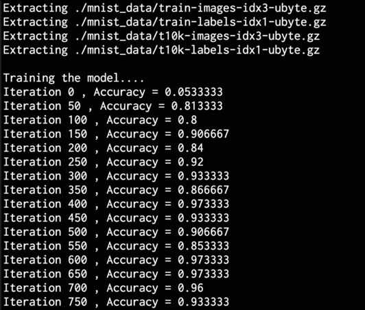

继续迭代时,精度会不断增加,如以下屏幕截图所示:
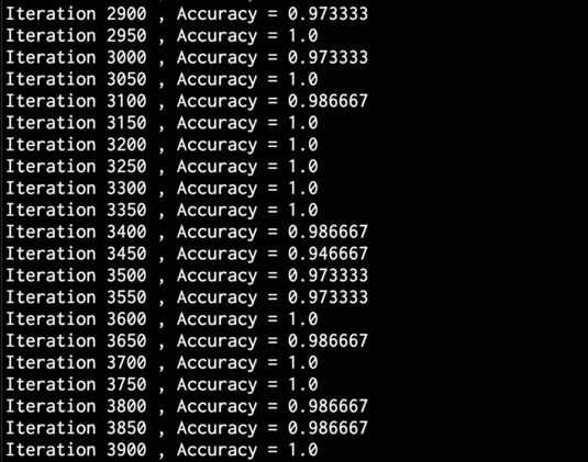

现在得到了输出,可以看到卷积神经网络的准确性远远高于简单的神经网络。

留言 点赞 关注
我们一起分享AI学习与发展的干货
欢迎关注全平台AI垂类自媒体 “读芯术”