有关语义分割的奇技淫巧有哪些？

2019 年 1 月 16 日 极市平台

极市平台（ExtremeMart）是深圳极视角旗下的专业视觉算法开发与分发平台，为开发者提供行业场景集，每月上百真实项目需求，算法分发，技术共享等，旨在联合开发者建立起良好的计算机视觉生态。已与上百名开发者建立了合作并转化了上百种视觉算法。

PS.本周四（1月17日）晚，国防科技大学助理研究员张钊宁博士，将为我们分享算力限制下的目标检测实战及思考，公众号回复“38”即可获取直播详情。

作者：AlexL

来源：https://www.zhihu.com/question/272988870/answer/562262315

知乎问题：有关语义分割的奇技淫巧有哪些？

AlexL的回答：

代码取自在Kaggle论坛上看到的帖子和个人做过的project

1. 如何去优化IoU

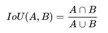
在分割中我们有时会去用intersection over union去衡量模型的表现，具体定义如下：

在有了这个定义以后我们可以规定比如说对于predicted instance和actual instance，IoU大于0.5算一个positive。在这基础之上可以做一些F1，F2之类其他的更宏观的metric。

所以说怎么去优化IoU呢？¬_¬

拿二分类问题举例，做baseline的时先扔上个binary-crossentropy看下效果，于是就有了以下的实现（PyTorch）：

class BCELoss2d(nn.Module):
     def __init__(self, weight=None, size_average=True):
         super(BCELoss2d, self).__init__()
         self.bce_loss = nn.BCELoss(weight, size_average)

     def forward(self, logits, targets):
         probs        = F.sigmoid(logits)
         probs_flat   = probs.view (-1)
         targets_flat = targets.view(-1)
         return self.bce_loss(probs_flat, targets_flat)

但是问题在于，优化BCE不等价于优化IoU。这篇文章（arxiv.org/pdf/1705.08790.pdf）说的显然比我要好，但是直观来说在一个minibatch里每个pixel的权重其实是不一样的。两张图片，一张正样本有1000个pixels，另一张只有4个，第二张一个pixel带来的IoU损失就能顶得上第一张中250个pixel的损失。

“那能不能直接优化IoU？“

可以，但这肯定不是最优的：

def iou_coef(y_true, y_pred, smooth=1):
    """    IoU = (|X &amp; Y|)/ (|X or Y|)    """
    intersection = K.sum(K.abs(y_true * y_pred), axis=-1)
    union = K.sum((y_true,-1) + K.sum(y_pred,-1) - intersection
    return (intersection + smooth) / ( union + smooth)def iou_coef_loss(y_true, y_pred):
    return -iou_coef(y_true, y_pred)

这次的问题在于训练过程的不稳定。一个模型从坏到好，我们希望监督它的loss/metric的过渡是平滑的，但直接暴力套用IoU显然不行。。。。

于是我们有了Lovász-Softmax！A tractable surrogate for the optimization of the intersection-over-union measure in neural networks：

https://github.com/bermanmaxim/LovaszSoftmax

具体为什么这个loss比BCE/Jaccard要好我不敢瞎说......但从个人使用体验来看效果拔群 \ (•◡•) /

还有一个很有意思的细节是：原implementation中这一段：

loss = torch.dot(F.relu(errors_sorted), Variable(grad))

如果把relu换成elu+1的话，有时效果更好。我猜测可能是因为elu+1比relu更平滑一些？

1.1 如果你不在乎训练时间的话

试试这个：

def symmetric_lovasz(outputs, targets):
        return (lovasz_hinge(outputs, targets) + lovasz_hinge(-outputs, 1 - targets)) / 2

1.2 如果你的模型斗不过Hard Examples的话

在你的loss后面加上这个：

def focal_loss(self, output, target, alpha, gamma, OHEM_percent):
        output = output.contiguous().view(-1)
        target = target.contiguous().view(-1)

        max_val = (-output).clamp(min=0)
        loss = output - output * target + max_val + ((-max_val).exp() + (-output - max_val).exp()).log()

        # This formula gives us the log sigmoid of 1-p if y is 0 and of p if y is 1
        invprobs = F.logsigmoid(-output * (target * 2 - 1))
        focal_loss = alpha * (invprobs * gamma).exp() * loss

        # Online Hard Example Mining: top x% losses (pixel-wise). Refer to http://www.robots.ox.ac.uk/~tvg/publications/2017/0026.pdf
        OHEM, _ = focal_loss.topk(k=int(OHEM_percent * [*focal_loss.shape][0]))
        return OHEM.mean()

2. 魔改U-Net

原始Unet长这样子（Keras)：

def conv_block(neurons, block_input, bn=False, dropout=None):
    conv1 = Conv2D(neurons, (3,3), padding='same', kernel_initializer='glorot_normal')(block_input)
    if bn:
        conv1 = BatchNormalization()(conv1)
    conv1 = Activation('relu')(conv1)
    if dropout is not None:
        conv1 = SpatialDropout2D(dropout)(conv1)
    conv2 = Conv2D(neurons, (3,3), padding='same', kernel_initializer='glorot_normal')(conv1)
    if bn:
        conv2 = BatchNormalization()(conv2)
    conv2 = Activation('relu')(conv2)
    if dropout is not None:
        conv2 = SpatialDropout2D(dropout)(conv2)
    pool = MaxPooling2D((2,2))(conv2)
    return pool, conv2  # returns the block output and the shortcut to use in the uppooling blocksdef middle_block(neurons, block_input, bn=False, dropout=None):
    conv1 = Conv2D(neurons, (3,3), padding='same', kernel_initializer='glorot_normal')(block_input)
    if bn:
        conv1 = BatchNormalization()(conv1)
    conv1 = Activation('relu')(conv1)
    if dropout is not None:
        conv1 = SpatialDropout2D(dropout)(conv1)
    conv2 = Conv2D(neurons, (3,3), padding='same', kernel_initializer='glorot_normal')(conv1)
    if bn:
        conv2 = BatchNormalization()(conv2)
    conv2 = Activation('relu')(conv2)
    if dropout is not None:
        conv2 = SpatialDropout2D(dropout)(conv2)
    
    return conv2def deconv_block(neurons, block_input, shortcut, bn=False, dropout=None):
    deconv = Conv2DTranspose(neurons, (3, 3), strides=(2, 2), padding="same")(block_input)
    uconv = concatenate([deconv, shortcut])
    uconv = Conv2D(neurons, (3, 3), padding="same", kernel_initializer='glorot_normal')(uconv)
    if bn:
        uconv = BatchNormalization()(uconv)
    uconv = Activation('relu')(uconv)
    if dropout is not None:
        uconv = SpatialDropout2D(dropout)(uconv)
    uconv = Conv2D(neurons, (3, 3), padding="same", kernel_initializer='glorot_normal')(uconv)
    if bn:
        uconv = BatchNormalization()(uconv)
    uconv = Activation('relu')(uconv)
    if dropout is not None:
        uconv = SpatialDropout2D(dropout)(uconv)
        
    return uconvdef build_model(start_neurons, bn=False, dropout=None):    
    input_layer = Input((128, 128, 1))
    # 128 -> 64
    conv1, shortcut1 = conv_block(start_neurons, input_layer, bn, dropout)
    # 64 -> 32
    conv2, shortcut2 = conv_block(start_neurons * 2, conv1, bn, dropout)
    # 32 -> 16
    conv3, shortcut3 = conv_block(start_neurons * 4, conv2, bn, dropout)
    # 16 -> 8
    conv4, shortcut4 = conv_block(start_neurons * 8, conv3, bn, dropout)   
    #Middle
    convm = middle_block(start_neurons * 16, conv4, bn, dropout)   
    # 8 -> 16
    deconv4 = deconv_block(start_neurons * 8, convm, shortcut4, bn, dropout)  
    # 16 -> 32
    deconv3 = deconv_block(start_neurons * 4, deconv4, shortcut3, bn, dropout)   
    # 32 -> 64
    deconv2 = deconv_block(start_neurons * 2, deconv3, shortcut2, bn, dropout)
    # 64 -> 128
    deconv1 = deconv_block(start_neurons, deconv2, shortcut1, bn, dropout)  
    #uconv1 = Dropout(0.5)(uconv1)
    output_layer = Conv2D(1, (1,1), padding="same", activation="sigmoid")(deconv1) 
    model = Model(input_layer, output_layer)
    return model

但一般与其是用transposed convolution我们会选择用upsampling+3*3 conv，具体原因请见这篇文章：Deconvolution and Checkerboard Artifacts （强烈安利distill，blog质量奇高）

再往下说，在实际做project的时候往往没有那么多的训练资源，所以我们得想办法把那些classification预训练模型嵌入到Unet中。ʕ•ᴥ•ʔ

把encoder替换预训练的模型的诀窍在于，如何很好的提取出pretrained models在不同尺度上提取出来的信息，并且如何把它们高效的接在decoder上。常见的用于嫁接的模型有Inception和Mobilenet，但我在这里就分析一下更直观一些的ResNet/ResNeXt这一类的模型：

def forward(self, x):
        x = self.conv1(x)
        x = self.bn1(x)
        x = self.relu(x)
        x = self.maxpool(x)

        x = self.layer1(x)
        x = self.layer2(x)
        x = self.layer3(x)
        x = self.layer4(x)

        x = self.avgpool(x)
        x = x.view(x.size(0), -1)
        x = self.fc(x)

        return x

我们可以很明显的看出不同尺度的feature map分别是由不同的layer来提取的，我们就可以从中选出几个来做concat，upsample，conv。唯一一点要注意的是千万不要错位concat，否则最后出来的output可能会和输入图大小不同。下面分享一个可行的搭法，其中为了提升各feature map的resolution我移去了原resnet conv1中的pool：

    def __init__(self):
        super().__init__()
        self.resnet = models.resnet34(pretrained=True)

        self.conv1 = nn.Sequential(
            self.resnet.conv1,
            self.resnet.bn1,
            self.resnet.relu,
        )

        self.encoder2 = self.resnet.layer1 # 64
        self.encoder3 = self.resnet.layer2 #128
        self.encoder4 = self.resnet.layer3 #256
        self.encoder5 = self.resnet.layer4 #512

        self.center = nn.Sequential(
            ConvBn2d(512,512,kernel_size=3,padding=1),
            nn.ReLU(inplace=True),
            ConvBn2d(512,256,kernel_size=3,padding=1),
            nn.ReLU(inplace=True),
            nn.MaxPool2d(kernel_size=2,stride=2),
        )

        self.decoder5 = Decoder(256+512,512,64)
        self.decoder4 = Decoder(64 +256,256,64)
        self.decoder3 = Decoder(64 +128,128,64)
        self.decoder2 = Decoder(64 +64 ,64 ,64)
        self.decoder1 = Decoder(64     ,32 ,64)

        self.logit = nn.Sequential(
            nn.Conv2d(384, 64, kernel_size=3, padding=1),
            nn.ELU(inplace=True),
            nn.Conv2d(64, 1, kernel_size=1, padding=0),
        )

    def forward(self, x):
        mean=[0.485, 0.456, 0.406]
        std=[0.229,0.224,0.225]
        x=torch.cat([
           (x-mean[2])/std[2],
           (x-mean[1])/std[1],
           (x-mean[0])/std[0],
        ],1)

        e1 = self.conv1(x)
        e2 = self.encoder2(e1)
        e3 = self.encoder3(e2)
        e4 = self.encoder4(e3)
        e5 = self.encoder5(e4)

        f = self.center(e5)
        d5 = self.decoder5(f, e5)
        d4 = self.decoder4(d5,e4)
        d3 = self.decoder3(d4,e3)
        d2 = self.decoder2(d3,e2)
        d1 = self.decoder1(d2)

关于decoder的设计方法，还有两个可以参考的小技巧：

一是 Concurrent Spatial and Channel Squeeze & Excitation in Fully Convolutional Networks（https://distill.pub/2016/deconv-checkerboard/)，可以理解为是一种attention，用很少的参数来校准feature map，详情请见论文，但实现细节可参考以下的PyTorch代码：

class sSE(nn.Module):
    def __init__(self, out_channels):
        super(sSE, self).__init__()
        self.conv = ConvBn2d(in_channels=out_channels,out_channels=1,kernel_size=1,padding=0)
    def forward(self,x):
        x=self.conv(x)
        #print('spatial',x.size())
        x=F.sigmoid(x)
        return xclass cSE(nn.Module):
    def __init__(self, out_channels):
        super(cSE, self).__init__()
        self.conv1 = ConvBn2d(in_channels=out_channels,out_channels=int(out_channels/2),kernel_size=1,padding=0)
        self.conv2 = ConvBn2d(in_channels=int(out_channels/2),out_channels=out_channels,kernel_size=1,padding=0)
    def forward(self,x):
        x=nn.AvgPool2d(x.size()[2:])(x)
        #print('channel',x.size())
        x=self.conv1(x)
        x=F.relu(x)
        x=self.conv2(x)
        x=F.sigmoid(x)
        return xclass Decoder(nn.Module):
    def __init__(self, in_channels, channels, out_channels):
        super(Decoder, self).__init__()
        self.conv1 = ConvBn2d(in_channels, channels, kernel_size=3, padding=1)
        self.conv2 = ConvBn2d(channels, out_channels, kernel_size=3, padding=1)
        self.spatial_gate = sSE(out_channels)
        self.channel_gate = cSE(out_channels)

    def forward(self, x, e=None):
        x = F.upsample(x, scale_factor=2, mode='bilinear', align_corners=True)
        #print('x',x.size())
        #print('e',e.size())
        if e is not None:
            x = torch.cat([x,e],1)

        x = F.relu(self.conv1(x),inplace=True)
        x = F.relu(self.conv2(x),inplace=True)
        #print('x_new',x.size())
        g1 = self.spatial_gate(x)
        #print('g1',g1.size())
        g2 = self.channel_gate(x)
        #print('g2',g2.size())
        x = g1*x + g2*x
        return x

还有一个就是为了进一步鼓励模型在多尺度上的鲁棒性，我们可以引入Hypercolumn(https://arxiv.org/pdf/1411.5752.pdf)去直接把各个scale的feature map concatenate起来：

f = torch.cat((
            F.upsample(e1,scale_factor= 2, mode='bilinear',align_corners=False),
            d1,
            F.upsample(d2,scale_factor= 2, mode='bilinear',align_corners=False),
            F.upsample(d3,scale_factor= 4, mode='bilinear',align_corners=False),
            F.upsample(d4,scale_factor= 8, mode='bilinear',align_corners=False),
            F.upsample(d5,scale_factor=16, mode='bilinear',align_corners=False),
        ),1)f = F.dropout2d(f,p=0.50)logit = self.logit(f)

更神奇的方法就是直接把每个scale的feature map和downsized gt进行比较计算loss，最后各个尺度的loss进行加权平均。详情请见这里的讨论：Deep semi-supervised learning | Kaggle

(https://www.kaggle.com/c/tgs-salt-identification-challenge/discussion/63715)这里就不再赘述了。

3. Training

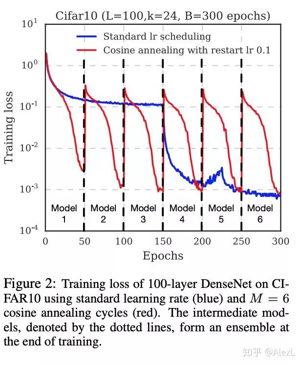
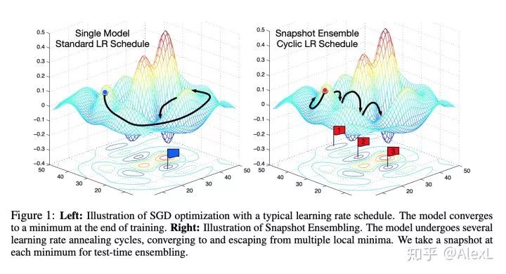
其实训练我觉得真的是case by case，在task A上用的heuristics放到task B效果就反而没那么好，所以我就介绍一个大多场合下都能用的trick：Cosine Annealing w. Snapshot Ensemble (https://arxiv.org/abs/1704.00109)

听上去听酷炫的，实际上就是每个一段时间warm restart学习率，这样在单位时间内能得到多个而不是一个converged local minina，做融合的话手上的模型会多很多。放几张图上来感受一下：

实现的话，其实挺简单的：

CYCLE=8000LR_INIT=0.1LR_MIN=0.001scheduler = lambda x: ((LR_INIT-LR_MIN)/2)*(np.cos(PI*(np.mod(x-1,CYCLE)/(CYCLE)))+1)+LR_MIN

然后每个batch/epoch去用scheduler(iteration)去更新学习率就可以了

4. 其他的一些小tricks（持续更新）

目前能想到的就是DSB2018 第一名的solution。与其是用mask rcnn去做instance segmentation，他们选择了U-Net生成class probability map+watershed小心翼翼分离离得比较近的instances。最后也是取得了领先第二名一截的成绩。不得不说有时候比起研究模型，研究数据并精炼出关键的insight往往能带来更多的收益......

最后安利一下我自己的repo： liaopeiyuan/ml-arsenal-public

(https://github.com/liaopeiyuan/ml-arsenal-public)，里面会有我所有参与过的Kaggle竞赛的源代码，目前有两个Top 1% solution：TGS Salt和Quick Draw Doodle。欢迎大家提issues/pull requests! XD

*推荐阅读*