
DGL学习(五): DGL构建异质图
使用dgl.heterograph()构建异质图,其参数是一个字典,key是一个三元组(srctype , edgetype, dsttype), 这个三元组被称为规范边类型( canonical edge types)。value 是一堆源数组和目标数组。节点是从零开始的整数ID, 不同类型的节点ID具有单独的计数。
import numpy as np
import dgl
import scipy.sparse as sp
import networkx as nx

ratings = dgl.heterograph(
    {('user', '+1', 'movie') : (np.array([0, 0, 1]), np.array([0, 1, 0])),
     ('user', '-1', 'movie') : (np.array([2]), np.array([1]))})
也可以从稀疏矩阵/networkX构造异质图。
## 从稀疏矩阵构造图
plus1 = sp.coo_matrix(([1, 1, 1], ([0, 0, 1], [0, 1, 0])), shape=(3, 2))
minus1 = sp.coo_matrix(([1], ([2], [1])), shape=(3, 2))
ratings = dgl.heterograph(
    {('user', '+1', 'movie') : plus1,
     ('user', '-1', 'movie') : minus1})

## 从networkX构造图
plus1 = nx.DiGraph()
plus1.add_nodes_from(['u0', 'u1', 'u2'], bipartite=0)
plus1.add_nodes_from(['m0', 'm1'], bipartite=1)
plus1.add_edges_from([('u0', 'm0'), ('u0', 'm1'), ('u1', 'm0')])
ratings = dgl.heterograph(
    {('user', '+1', 'movie') : plus1,
     ('user', '-1', 'movie') : minus1})
使用ACM异质图数据集:
import scipy.io
import urllib.request

data_url = 'https://data.dgl.ai/dataset/ACM.mat'
data_file_path = '/tmp/ACM.mat'

urllib.request.urlretrieve(data_url, data_file_path)
data = scipy.io.loadmat(data_file_path)
print(list(data.keys()))
['__header__', '__version__', '__globals__', 'TvsP', 'PvsA', 'PvsV', 'AvsF', 'VvsC', 'PvsL', 'PvsC', 'A', 'C', 'F', 'L', 'P', 'T', 'V', 'PvsT', 'CNormPvsA', 'RNormPvsA', 'CNormPvsC', 'RNormPvsC', 'CNormPvsT', 'RNormPvsT', 'CNormPvsV', 'RNormPvsV', 'CNormVvsC', 'RNormVvsC', 'CNormAvsF', 'RNormAvsF', 'CNormPvsL', 'RNormPvsL', 'stopwords', 'nPvsT', 'nT', 'CNormnPvsT', 'RNormnPvsT', 'nnPvsT', 'nnT', 'CNormnnPvsT', 'RNormnnPvsT', 'PvsP', 'CNormPvsP', 'RNormPvsP']
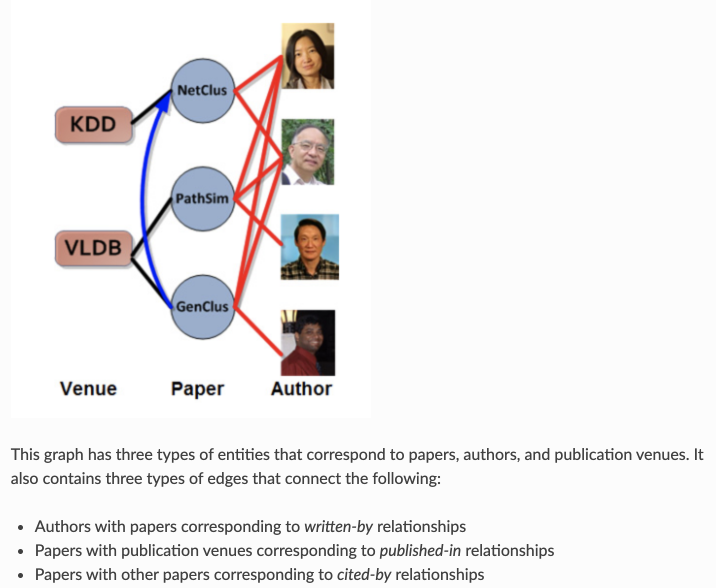
A代表作者, P代表论文, C代表会议,L是主题代码; 边存储为键XvsY下的SciPy稀疏矩阵,其中X和Y可以是任何节点类型代码。
输出PvsA (paper - author) 的一些统计量。
print(type(data['PvsA']))
print('#Papers:', data['PvsA'].shape[0])
print('#Authors:', data['PvsA'].shape[1])
print('#Links:', data['PvsA'].nnz)
转化Scipy Matrix 为 dgl.heterograph()。
pa_g = dgl.heterograph({('paper', 'written-by', 'author') : data['PvsA']})
# equivalent (shorter) API for creating heterograph with two node types:
pa_g = dgl.bipartite(data['PvsA'], 'paper', 'written-by', 'author')
打印出类型名称和其他结构信息。
print('Node types:', pa_g.ntypes)
print('Edge types:', pa_g.etypes)
print('Canonical edge types:', pa_g.canonical_etypes)

# 节点和边都是从零开始的整数ID,每种类型都有其自己的计数。要区分不同类型的节点和边缘,需要指定类型名称作为参数。
print(pa_g.number_of_nodes('paper'))

# 如果规范边类型名称是唯一可区分的,则可以将其简化为边类型名称。
print(pa_g.number_of_edges(('paper', 'written-by', 'author')))
print(pa_g.number_of_edges('written-by'))
## 获得论文#1 的作者
print(pa_g.successors(1, etype='written-by'))
Node types: ['paper', 'author']
Edge types: ['written-by']
Canonical edge types: [('paper', 'written-by', 'author')]
12499
37055
37055
tensor([3532, 6421, 8516, 8560])
Metagraph
## Metagraph(或网络模式)是异质图结构的一个概览。 被用作异质图的模板,它描述了网络中存在多少种对象以及可能存在的链接。
print(G.metagraph)
Graph(num_nodes={'author': 17431, 'paper': 12499, 'subject': 73},
      num_edges={('paper', 'written-by', 'author'): 37055, ('author', 'writing', 'paper'): 37055, ('paper', 'citing', 'paper'): 30789, ('paper', 'cited', 'paper'): 30789, ('paper', 'is-about', 'subject'): 12499, ('subject', 'has', 'paper'): 12499},
      metagraph=[('author', 'paper'), ('paper', 'author'), ('paper', 'paper'), ('paper', 'paper'), ('paper', 'subject'), ('subject', 'paper')])
半监督节点分类(Relational-GCN)
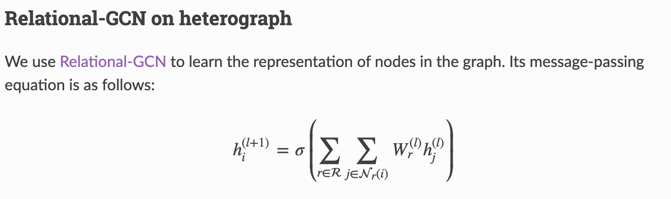
搭建异质图神经网络:
import dgl.function as fn

class HeteroRGCNLayer(nn.Module):
    def __init__(self, in_size, out_size, etypes):
        super(HeteroRGCNLayer, self).__init__()
        # W_r for each relation
        self.weight = nn.ModuleDict({
                name : nn.Linear(in_size, out_size) for name in etypes
            })

    def forward(self, G, feat_dict):
        # The input is a dictionary of node features for each type
        funcs = {}
        for srctype, etype, dsttype in G.canonical_etypes:
            # 计算每一类etype的 W_r * h
            Wh = self.weight[etype](feat_dict[srctype])
            # Save it in graph for message passing
            G.nodes[srctype].data['Wh_%s' % etype] = Wh
            # 消息函数 copy_u: 将源节点的特征聚合到'm'中; reduce函数: 将'm'求均值赋值给 'h'
            funcs[etype] = (fn.copy_u('Wh_%s' % etype, 'm'), fn.mean('m', 'h'))
        # Trigger message passing of multiple types.
        # The first argument is the message passing functions for each relation.
        # The second one is the type wise reducer, could be "sum", "max",
        # "min", "mean", "stack"
        G.multi_update_all(funcs, 'sum')
        # return the updated node feature dictionary
        return {ntype : G.nodes[ntype].data['h'] for ntype in G.ntypes}
class HeteroRGCN(nn.Module):
    def __init__(self, G, in_size, hidden_size, out_size):
        super(HeteroRGCN, self).__init__()
        # Use trainable node embeddings as featureless inputs.
        embed_dict = {ntype : nn.Parameter(torch.Tensor(G.number_of_nodes(ntype), in_size))
                      for ntype in G.ntypes}
        for key, embed in embed_dict.items():
            nn.init.xavier_uniform_(embed)
        self.embed = nn.ParameterDict(embed_dict)
        # create layers
        self.layer1 = HeteroRGCNLayer(in_size, hidden_size, G.etypes)
        self.layer2 = HeteroRGCNLayer(hidden_size, out_size, G.etypes)

    def forward(self, G):
        h_dict = self.layer1(G, self.embed)
        h_dict = {k : F.leaky_relu(h) for k, h in h_dict.items()}
        h_dict = self.layer2(G, h_dict)
        # get paper logits
        return h_dict['paper']
Train and evaluate
model = HeteroRGCN(G, 10, 10, 3)

opt = torch.optim.Adam(model.parameters(), lr=0.01, weight_decay=5e-4)

best_val_acc = 0
best_test_acc = 0

for epoch in range(100):
    logits = model(G)
    # The loss is computed only for labeled nodes.
    loss = F.cross_entropy(logits[train_idx], labels[train_idx])

    pred = logits.argmax(1)
    train_acc = (pred[train_idx] == labels[train_idx]).float().mean()
    val_acc = (pred[val_idx] == labels[val_idx]).float().mean()
    test_acc = (pred[test_idx] == labels[test_idx]).float().mean()

    if best_val_acc < val_acc:
        best_val_acc = val_acc
        best_test_acc = test_acc

    opt.zero_grad()
    loss.backward()
    opt.step()

    if epoch % 5 == 0:
        print('Loss %.4f, Train Acc %.4f, Val Acc %.4f (Best %.4f), Test Acc %.4f (Best %.4f)' % (
            loss.item(),
            train_acc.item(),
            val_acc.item(),
            best_val_acc.item(),
            test_acc.item(),
            best_test_acc.item(),
        ))

