![[新手]从Linear到LSTM,5种方法由浅入深预测股价](data:image/svg+xml;utf8,<svg xmlns='http://www.w3.org/2000/svg'></svg>)
[新手]从Linear到LSTM,5种方法由浅入深预测股价

机器学习在股票价格预测上的应用
机器学习有非常多的实际应用,其中包含时间序列预测。其中最有趣或者说最有利可图的可以说是股票价格预测了。
问题描述:
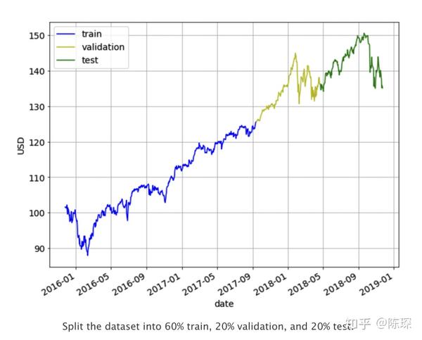
问题的目标是使用前N天的数据,预测每日调整收盘价。我们使用近3年的历史价格数据(2015-11-25 to 2018-11-23)来进行训练。
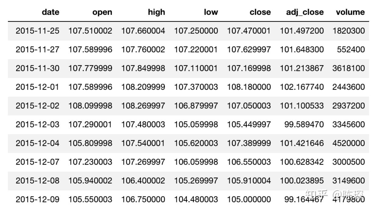
数据集看起来像这样:

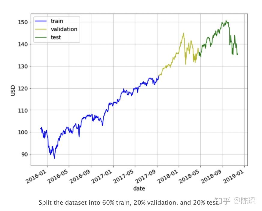
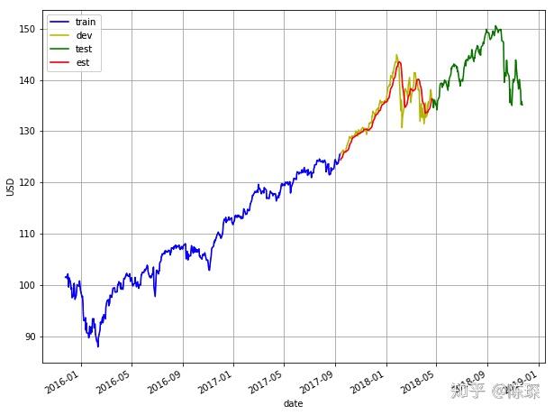
我们将数据集拆分为60%的train set,20%的validation set,20%的test set。使用train set进行模型的训练,通过观察在validation set上的效果调整超参数,最终模型的性能将在test上进行评估。切分如下图所示:
评估模型效果使用的指标为RMSE(mean square error)和MAPE(mean absolute percentage error)。对于这两个指标,值越低则模型效果越好。
Last Value
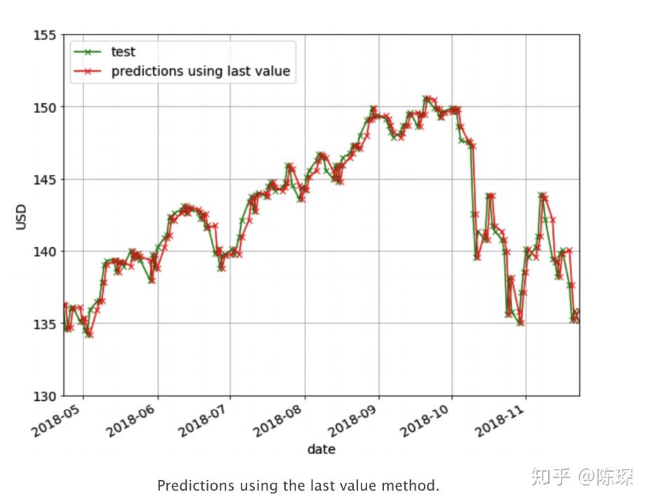
在Last Value方法中,我们只需要将预测值设置为最后一个观察值。我们仅需要设置当天的收盘价为前一天的收盘价。这个方法作为我们的benchmark方法来与一些较为复杂的模型做性能比较。它没有需要训练的参数,是一个成本很低的预测模型。 下图是使用Last Value的预测结果。

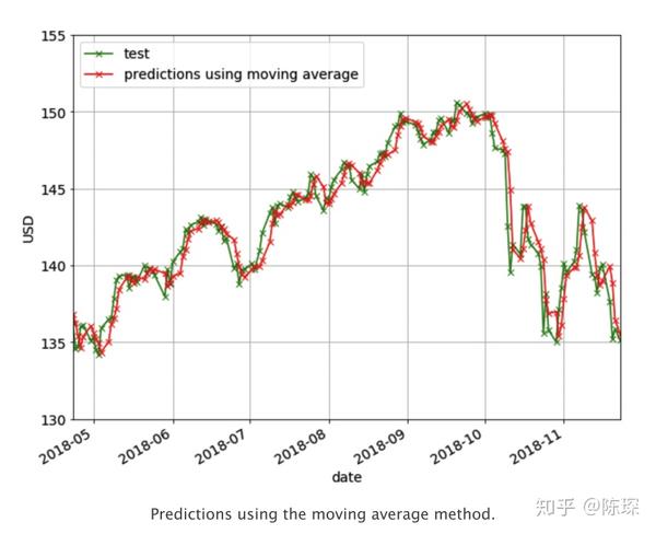
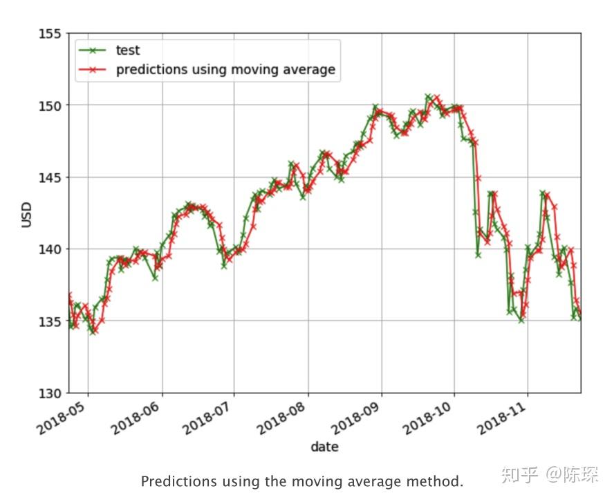
Moving Average
在moving average方法中,预测是前N天的调整后收盘价的平均值,N的选取需要进行学习调整。 基于moving average方法计算了不同N值取值对应的RMSE值,如下图:

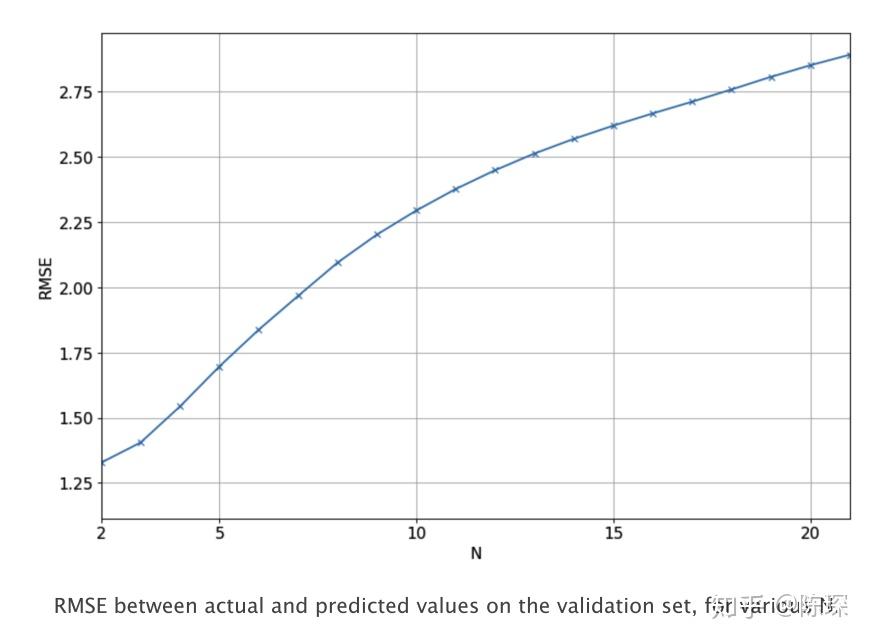
对应N=2的moving average方法效果如下:
Linear Regression
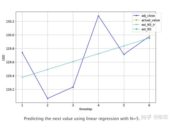
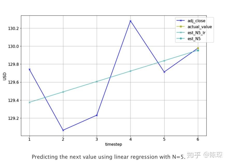
线性回归是对一个或多个独立变量之间线性关系建模的方法。我们使用线性回归模型拟合前N天收盘价,得到一个模型后对当天的收盘价进行预测。下图为N=5时的一个例子,实际调整后的收盘价为(蓝色+),需要预测第6天的收盘价格(黄色方形)。需要基于前5个实际值,拟合一个linear regression模型(浅蓝色线),对第6天进行预测(亮蓝色圈圈)。
下面是我们训练linear regression使用的代码:
import numpy as np
from sklearn.linear_model import LinearRegression
def get_preds_lin_reg(df, target_col, N, pred_min, offset):
"""
Given a dataframe,get prediction at each timestep
:param df: dataframe with the values you want to predict
:param target_col: name of the column you want to predict
:param N: use previous N values to do prediction
:param pred_min: all predictions should be >= pred_min
:param offset: for df we only do predictions for df[offset:]
:return: pred_list: the predictions for target_col
"""
# create linear regression object
regr = LinearRegression(fit_intercepter=True)
pred_list = []
for i in range(offset, len(df['adj_close'])):
X_train = np.array(range(len(df['adj_close'][i-N:i])))
y_train = np.array(df['adj_close'][i-N:i])
X_train = X_train.reshape(-1,1)
y_train = y_train.reshape(-1,1)
# train the model
regr.fit(X_train, y_train)
pred = regr.predict(N)
# If the values are < pred_min,set it to be pred_min
pred_list = np.array(pred_list)
pred_list[pred_list < pred_min] = pred_min
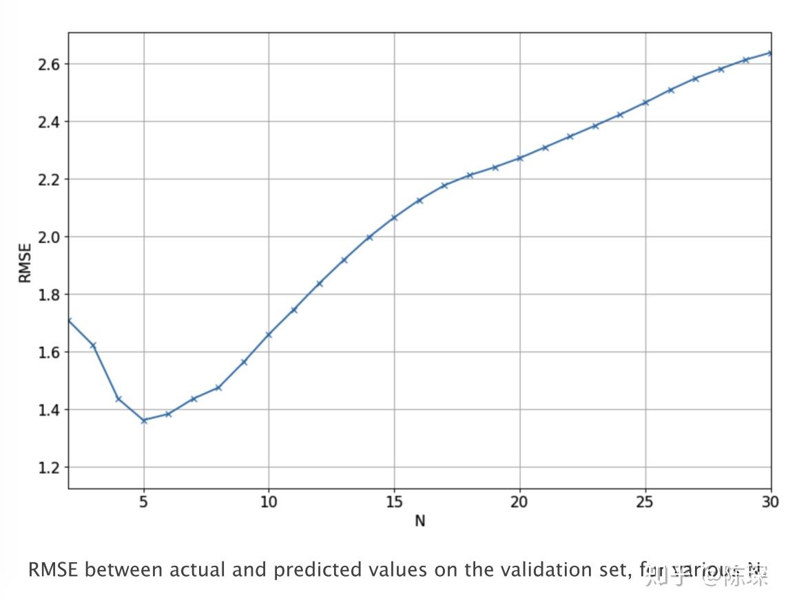
return pred_list下图显示了不同N的取值对应的模型在验证集上实际值与预测值之间的RMSE。我们最终选择N=5,因为它对应的RMSE是最低的。

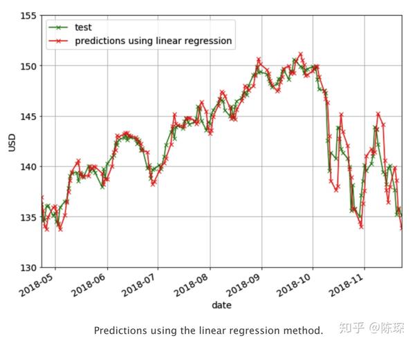
下面的曲线显示了N=5时的预测效果。但可以看出它也没有表达增长或下跌趋势的能力。
XGBoost
Gradient Boosting是以迭代的方式,不断学习残差,将一个弱模型变成一个强模型。XGBoost全称Extreme Gradient Boosting,指的是以压榨计算资源极限为目标的提升树算法。在2014年被提出后,在各大机器学习竞赛和实际项目中被广泛使用。
我们将在train set上训练模型,基于validation set来调整参数,并在test set上进行预测并输出预测结果,并进行RMSE的效果评估。在机器学习任务中一般称一列为一个特征,在我们之前的几个模型中仅使用到了当日调整收盘价本身。除了raw的特征列,针对当前的数据序列我们可以提取更多的特征来丰富对数据的表达。比如我们这里加入:
- 过去N天每天high与low的差异;
- 过去N天每天的open与close的差异;
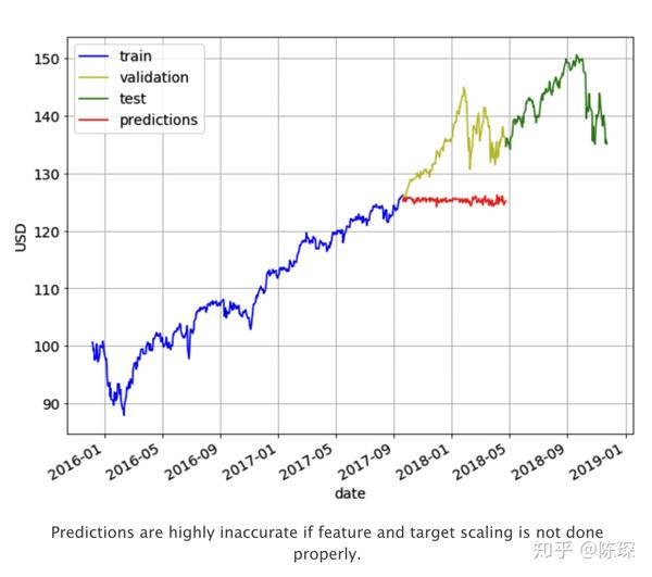
在构建这个模型的过程中可以体会到feature scaling对模型效果的影响程度。当你不做任何feature preprocessing,predictions在val set上表现极差,由于train set价格在89-125之间,模型预测也只能输出89-125之间的数字。而val set的价格远超出了该区间,模型是完全无法预测的。预测结果如下图红色。
接下来测试将train set的缩放到正态分布,也叫mean=0 & variance=1的高斯分布。同时在validation set上做一样的缩放操作。但是因为mean和variance我们都是在train set计算的,很明显这样操作的效果也不会很好。validation set上的数据比train set上的大很多,通过缩放后依然会很大。最后预测的结果依然如上图,区别只是输出的是缩放后的y值。
最后,首先依然将train set缩放到正态分布,并进行模型的训练。随后,在validation set上进行预测时,对应每一个特征列都将其放缩至正态分布。比如我们要对第T天进行预测,获取前N天的调整收盘价然后对其进行放缩。对于volume特征也是同样的操作。然后在每一个构建的特征上都重复同样的操作。然后我们使用这些缩放后的特征进行预测,那么得到的预测结果同样是缩放后的。最后我们需要使用对应的mean和variance对他们进行转换得到对应的实际值。该方法目前效果是最好的。 下面是我们训练XGBoost模型所使用的代码:
import math
import numpy as np

from sklearn.metrics import mean_squared_error
from xgboost import XGBRegressor

def get_mape(y_true, y_pred):
    """
    compute mean absolute percentage error (MAPE)
    :param y_true:
    :param y_pred:
    :return:
    """
    y_true, y_pred = np.array(y_true), np.array(y_pred)
    return np.mean(np.abs((y_true- y_pred) / y_true)) * 100

def train_pred_eval_model(X_train_scaled,
                          y_train_scaled,
                          X_test_scaled,
                          y_test,
                          col_mean,
                          col_std,
                          seed = 100,
                          n_estimators = 100,
                          max_depth = 3,
                          learning_rate = 0.1,
                          min_child_weight=1,
                          subsample = 1,
                          colsample_bytree=1,
                          colsample_bylevel=1,
                          gamma = 0):
    """
    train model,do prediction,scale back to original range and do evaluation
    :param X_train_scaled: features for training,Scaled to mean=0 & var = 1
    :param y_train_scaled: target for training.Scaled to have mean=0 & var=1
    :param X_test_scaled: features for test.Each sample is scaled to mean=0 and var=1
    :param y_test: target for test.Actual values, not scaled.
    :param col_mean: means used to scale each sample of X_test_scaled.
    same length as X_test_scaled and y_test
    :param col_std: standard deviations used to scale each sample of X_test_scaled.
    same length as X_test_scaled and y_test
    :param seed: model seed
    :param n_estimators: number of boosted trees to it
    :param max_depth: maximum tree depth for base learners
    :param learning_rate: boosting learning rate (xgb'eta)
    :param min_child_weight: minimum sum of instance weight needed in a child
    :param subsample: subsample ratio of the training instance
    :param colsample_bytree: subsample ratio of columns when constructing each tree
    :param colsample_bylevel: subsample ratio of columns for each split, in each level
    :param gamma: minimum loss reduction required to make a further partition on a leaf node of the tree
    :return:
    rmse:root mean square error of y_test and est
    mape:mean absolute percentage error of y_test and est
    est:predicted values.Same length as y_test.
    """
    model = XGBoostRegressor(seed=model_seed,
                             n_estimators=n_estimators,
                             max_depth=max_depth,
                             learning_rate=learning_rate,
                             min_child_weight=min_child_weight,
                             subsample=subsample,
                             colsample_bytree=colsample_bytree,
                             colsample_bylevel=colsample_bylevel,
                             gamma=gamma)
    # train the model
    model.fit(X_train_scaled,y_train_scaled)

    # get predicted labels and scale back to original range
    est_scaled = model.predict(X_test_scaled)
    est = est_scaled * col_std +  col_mean

    # calculate RMSE
    rmse = math.sqrt(mean_squared_error(y_test,est))
    mape = get_mape(y_test,est)
    return rmse,mape,est
在不同的N的取值下我们测试了val set上实际值与预测值对应的RMSE与MAPE值:
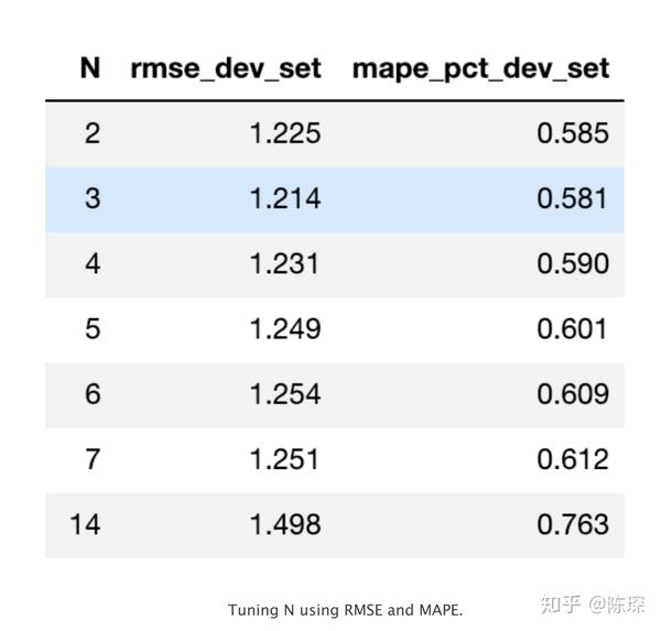
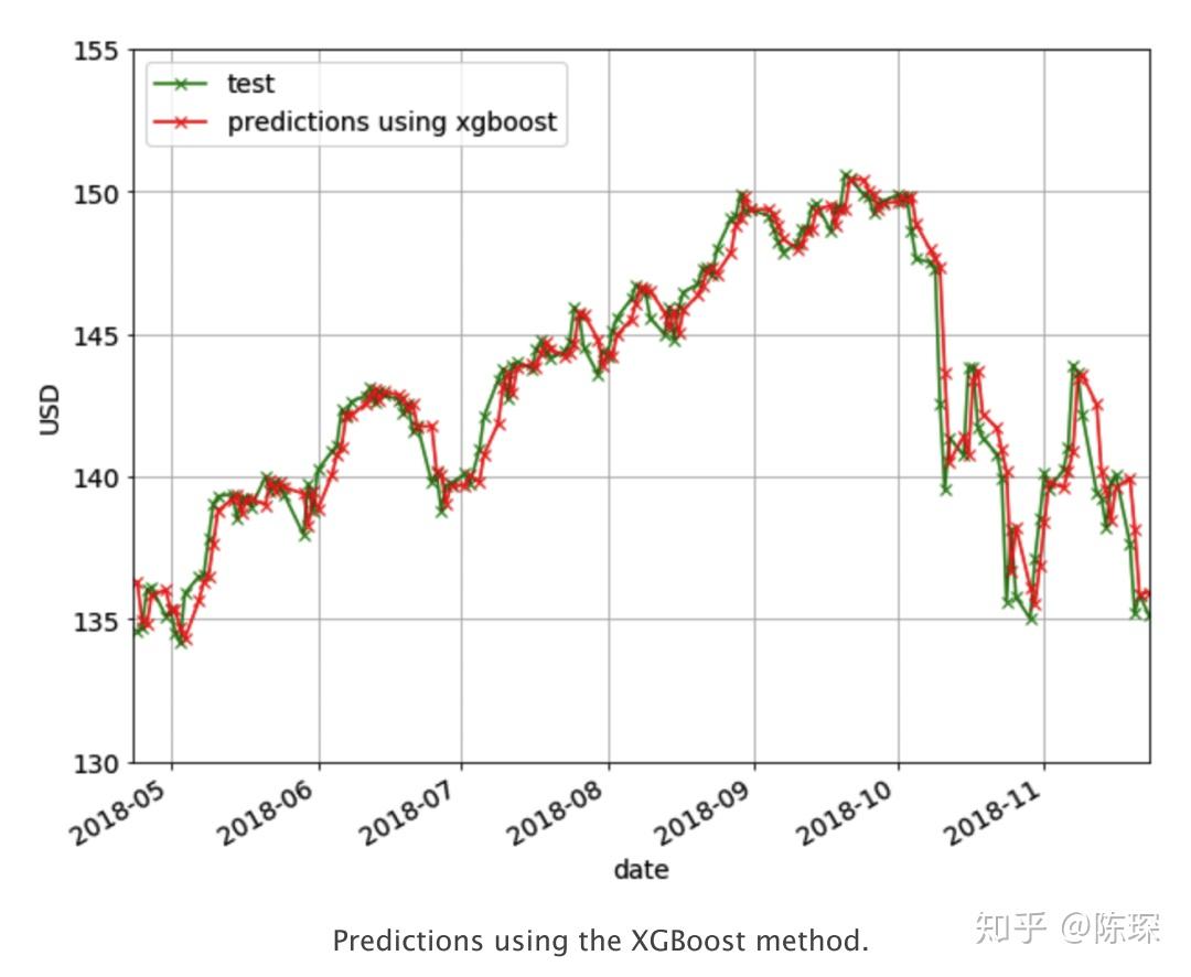
以RMSE为评估标准,则最好N = 3。对应的预测效果如下图:

LSTM
终于我们来到了LSTM!
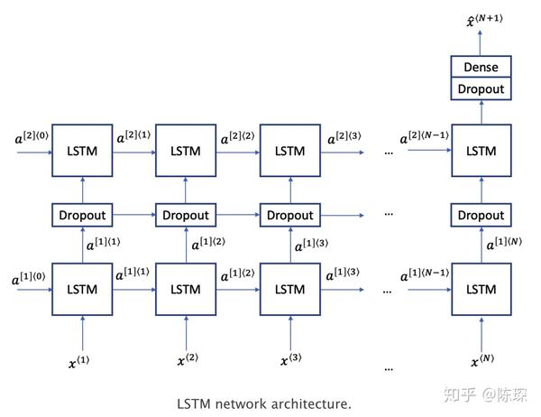
LSTM是一种为了对抗较长序列中遇到的梯度消失问题而设计的深度学习技术。LSTM有三种类型的门:记忆门,遗忘门,输出门。遗忘门与记忆门决定每个存储单元被更新。输出门决定了激活下一层的信息量。 LSTM的结构如下图,我们使用双层LSTM,介于之间的dropout layer用来防止过拟合。 更多有关于LSTM的信息,请移步李宏毅老师的课程。
下面是我们训练LSTM模型所使用的代码:
import math
import numpy as np

from keras.models import Sequential
from keras.layers import Dense,Dropout,LSTM

def train_pred_eval_model(x_train_scaled,
                          y_train_scaled,
                          x_test_scales,
                          y_test,
                          mu_test_list,
                          std_test_list,
                          lstm_units=50,
                          dropout_prob=0.5,
                          optimizer='adam',
                          epochs=1,
                          batch_size=1):
    """
    traim,prediction,scale back to original value,do evaluation
    :param x_train_scaled:
    :param y_train_scaled:
    :param x_test_scales:
    :param y_test:
    :param mu_test_list:list of means.Same length as y_test
    :param std_test_list:list of std devs.Same length as y_test
    :param lstm_units:dimensionality of the output space
    :param dropout_prob:fraction of the units to drop
    :param optimizer:optimizer for model.compile()
    :param epochs:epochs for model.fit()
    :param batch_size:batch size for model.fit()
    :return:
    rmse: root mean square error
    mape: mean absolute percentage error
    est:predictions
    """

    # create LSTM network
    model = Sequential()
    model.add(LSTM(units=lstm_units,
                   return_sequences=True,
                   input_shape=(x_train_scaled.shape[1],1)))

    # add dropout with a probability
    model.add(Dropout(dropout_prob))

    model.add(LSTM(units=lstm_units))

    # add dropout with a probability
    model.add(Dropout(dropout_prob))

    model.add(Dense(1))

    # compile and fit the LSTM network
    model.compile(loss='mean_squared_error',
                  optimizer=optimizer)
    model.fit(x_train_scaled,y_train_scaled,epochs=epochs,
              batch_size=batch_size,verbose=0)

    # Do prediction
    est_scaled = model.predict(x_test_scaled)
    est = (est_scaled * np.array(std_test_list).reshape(-1,1)) +
    np.array(mu_test_list).reshape(-1,1)

    # calculate RMSE and MAPE
    rmse = math.sqrt(mean_squared_error(y_test,est))
    mape = get_mape(y_test, est)
    return rmse,mape,est
下面是LSTM在val set上的结果:

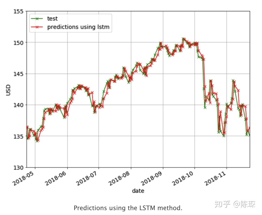
下面是基于LSTM预测的结果:

END
以上描述了:
- Last Value
- moving average
- linear regression
- XGBoost
- LSTM
但都是浅尝辄止,要依赖短短的分析获取收益是不可能的。
可能就像我们在不同的能力阶段看待同一个问题有不同的角度一样。
觉得有用有收获的话,关注我吧!