推荐系统系列（七）：NFM理论与实践

背景

传统FM模型虽然考虑了组合特征，但是其本质仍是一种线性模型，模型的表征能力终究是有限的。后续的Wide&Deep [3]、DeepCrossing [4]等模型在FM的基础上引入了DNN，试图加强模型的非线性能力，但这类模型对于参数较为敏感，训练难度较大。且在Wide&Deep等模型中，对于二阶交叉特征向量仅进行简单concatenation，然后送入后续DNN部分，将捕获高阶特征交叉信息的任务交给了DNN结构。这种简单拼接的方式，并没有将二阶交叉特征的信息完全表征出来，对于后续DNN来说，基于此结构学习更高阶交叉信息效率太低。

基于这些分析，新加坡国立大学于2017年提出Neural Factorization Machine（NFM）模型 [1]。同样是在FM的基础上引入DNN，利用非线性结构来学习更多数据信息。不同于Wide&Deep、DeepCrossing等模型，NFM使用Bi-Interaction Layer（Bi-linear interaction）结构来对二阶交叉信息进行处理，使交叉特征的信息能更好的被DNN结构学习，降低DNN学习更高阶交叉特征信息的难度。减轻DNN的负担，意味着不再需要更深的网络结构，从而模型参数量也减少了，模型训练更便捷。

分析

1. NFM 结构定义

NFM公式化定义如下：

\begin{aligned} \hat{y}_{NFM}(X)=w_0+\sum_{i=1}^{n}w_ix_i+f(X) \end{aligned} \qquad (1)

模型结构图如下所示，注意这个部分并未涵盖一阶项与偏置，完整的NFM是将三者涵盖其中的。
​

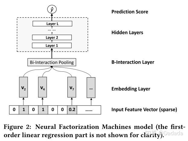
​从结构图可以看出NFM共有四个部分，下面分别对于每个部分进行详细讲解。

1.1 Embedding Layer

embedding vector的计算与之前介绍的模型保持一致，可通过lookup table获取。最终输入特征向量是由输入特征值 x_i 与 embedding vector v_i 相乘得到，即 V_x=\{x_1v_1,\dots,x_nv_n\} ​ 。个人认为这个部分与以前的模型没有区别。

1.2 Bi-Interaction Layer

Bi-Interaction Layer是NFM的核心，其本质是一个pooling操作，将embedding vector集合归并为一个向量。

\begin{aligned} f_{BI}(V_x)=\sum_{i=1}^n\sum_{j=i+1}^nx_iv_i \odot x_jv_j \end{aligned} \qquad (2)
其中， \odot ​ 表示两个向量对应元素相乘，其结果为一个向量。所以，Bi-Interation Layer将embedding vectors 进行两两交叉 ​ \odot 运算，然后将所有向量进行对应元素求和，最终 f_{BI}(V_x) ​ 为pooling之后的一个向量。
公式（2）的计算时间复杂度为 O(kn^2) ​ ，​ k 为embedding vector维度，类似于FM，可以对公式（2）进一步改写为：
\begin{aligned} f_{BI}(V_x)=\frac{1}{2}\left[\left(\sum_{i=1}^nx_iv_i\right)^2-\sum_{i=1}^n\left(x_iv_i\right)^2\right] \end{aligned} \qquad (3)
改写之后的时间复杂度为 ​ O(kN_x) ，其中 ​ N_x 为输入特征 ​ X 的非零元素个数。Bi-Interaction Layer与FM中的二阶交叉项相比，没有引入额外的参数，同时也能以线性时间复杂度进行训练，这是非常好的性质。

1.3 Hidden Layer

DNN部分的定义如下：

\begin{aligned} z1={}&\sigma_1(W_1f_{BI}(V_x)+b_1) \\ z2={}&\sigma_2(W_2z_1+b_2) \\ &\dots \dots \\ z_L={}&\sigma_L(W_Lz_{L-1}+b_L) \\ \end{aligned}
其中 W_l,b_l ​ 分别表示参数矩阵与偏置向量， \sigma ​ 表示激活函数，可以取 ​ sigmoid,tanh,relu 等。关于隐藏层的结构，可以使用类似于FNN中的几种结构： tower,constant,diamond ​ 等。

1.4 Prediction Layer

最后一层隐藏层加上一个线性变换，作为结果输出，即： f(X)=h^Tz_L ​ 。

最终，公式（1）可以表示为公式（4）

\begin{aligned} \hat{y}_{NFM}(X)={}&w_0+\sum_{i=1}^{n}w_ix_i+f(X) \\ ={}&w_0+\sum_{i=1}^{n}w_ix_i \\ +&h^T\sigma_L(W_L(\dots \sigma_1(W_1f_{BI}(V_x)+b_1)\dots)+b_L) \end{aligned} \qquad (4)

由此也可以看出，如果将中间的隐藏层去掉，仅保留最终的prediction layer，同时将 h ​ 设定为全1的向量，那么NFM完全复现了FM，可以认为NFM就是FM的推广。

a trainable h can not improve the expressiveness of FM, since its impact on prediction can be absorbed into feature embeddings.[1]

h 不会增强FM的表征能力，因为该参数可以吸收到特征的embedding 向量中。换句话说，就算 ​ h 不是全为1的向量，我们也可将其视为FM的等价模型。
仔细观察公式（4），上述Figure2的的结构图仅对应公式中的 ​ f(X) 项。如果将全局偏置 w_0 ​ 与一阶项 \sum_{i=1}^nw_ix_i ​ 综合考虑，其实NFM的结构图与Wide&Deep极为相似，但NFM中的二阶项与DNN是 串联结构 。 NFM左侧同样可以看做是一个LR模型，但不同于Wide&Deep，NFM左侧的LR模型仅输入单特征，并没有将组合特征送入LR模型，所以也就无需进行额外的特征工程工作。

2. 过拟合风险

将模型复杂度提高，不可避免的会面临训练过拟合的问题，NFM作者使用了dropout与batch normalization技术来缓解过拟合问题。后续实验表明，结合使用这两种技术能够有效的避免过拟合风险。

2.1 dropout

为了防止过拟合，可以使用dropout技术。需要注意的是，dropout一般是用于Bi-Interaction Layer输出之后，对于后续的每一层隐层都可使用。[5]

2.2 batch normalization

为了加速模型的收敛，同时还可使用batch normalization技术。同样的，作用于Bi-Interaction的输出，以及后续的隐层。[5]

2.3 附加层相对顺序

同时使用dropout，与batch normalization技术，需要注意两者的使用顺序。在 Batch Normalization: Accelerating Deep Network Training by Reducing Internal Covariate Shift 一文中，作者提到 :

we would like to ensure that for any parameter values, the network always produces activations with the desired distribution.[2]

也就是说，需要为激活函数提供需要的数据分布。所以，应该在Bi-Interaction Layer之后接入batch normalization，然后直接进行dropout。需要注意的是，Bi-Interaction Layer是没有激活函数的。后续隐层需要进行batch normalization调整数据分布，然后再加上激活函数，最后使用dropout技术。

3. 性能分析

个人认为NFM论文中对于模型的消融分析（Ablation study）做得非常精彩，值得大家一起来学习。

作者围绕三个问题对NFM的表现能力进行分析，下面一一来进行讲解。

3.1 问题一

Q：Bi-Interaction pooling 能否有效捕获二阶交叉特征信息？dropout与batch normalization能否起作用？

首先将NFM去除隐层，得到NFM-0模型，此时的NFM-0与FM等价。以LR作为对比模型，在不同dropout比例、不同的L2正则化强度下，NFM-0的表现如下：

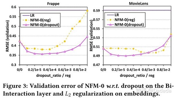
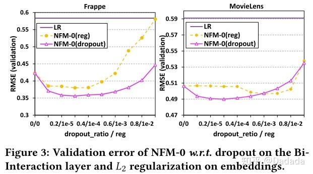
从上述实验可以看出，NFM-0比LR表现好很多，说明Bi-Interaction pooling能够捕获二阶交叉信息。dropout与L2正则对比可以说明，NFM-0更适合使用dropout技术。

下面对比试验，观察dropout是否能够有效缓解模型过拟合问题。

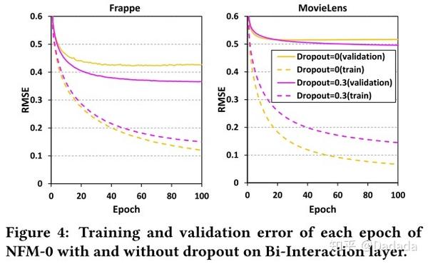
图4可以看出，dropout能够有效缓解模型过拟合问题。

接下来试验观察batch normalization的效果

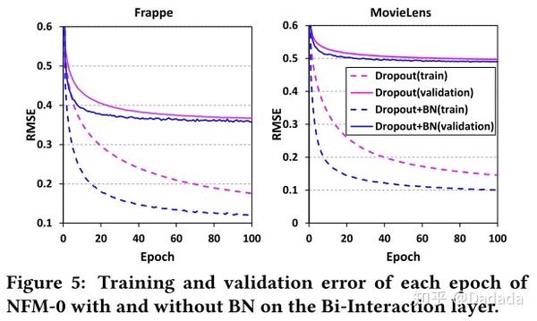
从图5可以看出，batch normalization能够明显加速模型收敛。同时可以看出，结合dropout与batch normalization技术能够有效避免过拟合，提高模型泛化能力。

3.2 问题二

Q：NFM隐层能否有效的捕获更高阶交叉特征信息？

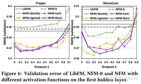
NFM使用一层隐层，同时将维度与Bi-Interaction的输出维度保持一致，对比NFM-0、FM（二者其实是等价的）有巨大提升。说明，NFM中的DNN部分能够学习更高阶交叉特征信息，帮助模型提效。

同时，对比不同的激活函数发现，引入非线性激活函数比线性函数（identity）表现更加优异。这也说明了非线性结构（DNN）的必要性。

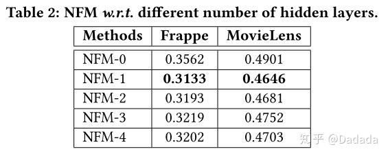
除此之外，作者还对隐层结构进行实验对比。首先比较了不同隐层带来的效果，如table2所示，NFM-1是最佳状态，继续叠加隐层反而效果会有所下降。说明NFM的Bi-Interaction能充分的捕获二阶交叉特征信息，所以只需要接入较浅的隐层结构就能捕获更高阶的信息，从而取得不错的效果。

We think the reason is because the Bi-Interaction layer has encoded informative second-order feature interactions, and based on which, a simple non-linear function is sufficient to capture higher-order interactions. [1]

为了进一步验证Bi-Interaction捕获信息的高效性，作者将Bi-Interaction替换为concatenation。实验结果发现，随着隐层结构越来越深，效果也会越来越好，但是最佳效果仍不如NFM-1。

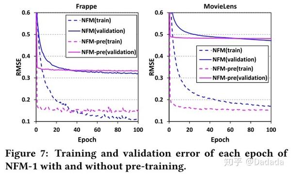
因为Wide&Deep、DeepCrossing使用FM预训练参数初始化时能够有更好的表现，为了更进一步展示NFM的优越性，作者还考察了NFM参数是否对于预训练敏感。

将FM训练得到的参数作为NFM的初始化参数，对比预训练模式与随机初始化模式的效果。从图7可以看出，预训练只能起到加速收敛的作用，对于最终的结果影响不大。而NFM对于参数初始化不敏感，更容易进行训练优化。

3.3 问题三

Q：NFM与目前（2017年）最好的模型（Wide&Deep、DeepCrossing）相比如何呢？

NFM使用一层隐层，激活函数为relu，与对比模型保持一致，dropout设置为0.5。Wide&Deep、DeepCrossing使用原论文中最佳参数。

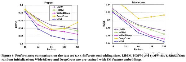
通过实验选择最佳的embedding 维度，如图8所示，除了DeepCrossing，其他模型的表现基本一致，所以最终选择128、256作为对比参数。

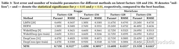
从最终的对比结果Table3来看，NFM的确表现最佳。除此之外也能够发现一些其他有意思的现象。

HOFM（使用了更高阶交叉特征的FM）与FM对比可以发现，更高阶的特征交叉能够带来提升，但HOFM采用线性方式拟合高阶特征，这种做法带来的提升效果有限，且模型参数更多。对比HOFM与NFM可以看出，使用非线性方式拟合高阶特征才能带来巨大提升效果，且NFM所引入的参数远远低于HOFM。

Wide&Deep与DeepCrossing在使用预训练的参数进行初始化之后，能够取得更好的效果。DeepCrossing使用了10层网络结构，但是最终的效果却不及FM，这说明DeepCrossing难以训练优化，网络并不是越深越好。

总而言之，NFM结构简单参数少，训练速度快（Bi-Interaction Layer的复杂度为 ​ ），效果棒！简直是居家旅行必备模型。

实践

NFM核心代码如下:

class NFM(object):
    def __init__(self, vec_dim=None, field_lens=None, dnn_layers=None, lr=None, dropout_rate=None):
        self.vec_dim = vec_dim
        self.field_lens = field_lens
        self.field_num = len(field_lens)
        self.dnn_layers = dnn_layers
        self.lr = lr
        self.dropout_rate = dropout_rate
        assert isinstance(dnn_layers, list) and dnn_layers[-1] == 1
        self._build_graph()

    def _build_graph(self):
        self.add_input()
        self.inference()

    def add_input(self):
        self.x = [tf.placeholder(tf.float32, name='input_x_%d'%i) for i in range(self.field_num)]
        self.y = tf.placeholder(tf.float32, shape=[None], name='input_y')
        self.is_train = tf.placeholder(tf.bool)

    def inference(self):
        with tf.variable_scope('linear_part'):
            w0 = tf.get_variable(name='bias', shape=[1], dtype=tf.float32)
            linear_w = [tf.get_variable(name='linear_w_%d'%i, shape=[self.field_lens[i]], dtype=tf.float32) for i in range(self.field_num)]
            linear_part = w0 + tf.reduce_sum(
                tf.concat([tf.reduce_sum(tf.multiply(self.x[i], linear_w[i]), axis=1, keep_dims=True) for i in range(self.field_num)], axis=1),
                axis=1, keep_dims=True) # (batch, 1)
        with tf.variable_scope('emb_part'):
            emb = [tf.get_variable(name='emb_%d'%i, shape=[self.field_lens[i], self.vec_dim], dtype=tf.float32) for i in range(self.field_num)]
            emb_layer = tf.concat([tf.matmul(self.x[i], emb[i]) for i in range(self.field_num)], axis=1) # (batch, F*K)
            emb_layer = tf.reshape(emb_layer, shape=(-1, self.field_num, self.vec_dim)) # (batch, F, K)
        with tf.variable_scope('bi_interaction_part'):
            sum_square_part = tf.square(tf.reduce_sum(emb_layer, axis=1)) # (batch, K)
            square_sum_part = tf.reduce_sum(tf.square(emb_layer), axis=1) # (batch, K)
            nfm = 0.5 * (sum_square_part - square_sum_part)
            nfm = tf.layers.batch_normalization(nfm, training=self.is_train, name='bi_interaction_bn')
            nfm = tf.layers.dropout(nfm, rate=self.dropout_rate, training=self.is_train)
        with tf.variable_scope('dnn_part'):
            in_node = self.vec_dim
            for i in range(len(self.dnn_layers)-1):
                out_node = self.dnn_layers[i]
                w = tf.get_variable(name='w_%d'%i, shape=[in_node, out_node], dtype=tf.float32)
                b = tf.get_variable(name='b_%d'%i, shape=[out_node], dtype=tf.float32)
                in_node = out_node
                nfm = tf.matmul(nfm, w) + b
                nfm = tf.layers.batch_normalization(nfm, training=self.is_train, name='bn_%d'%i)
                nfm = tf.nn.relu(nfm)
                nfm = tf.layers.dropout(nfm, rate=self.dropout_rate, training=self.is_train)
            h = tf.get_variable(name='h', shape=[in_node, 1], dtype=tf.float32)
            nfm = tf.matmul(nfm, h) # (batch, 1)

        self.y_logits = linear_part + nfm
        self.y_hat = tf.nn.sigmoid(self.y_logits)
        self.pred_label = tf.cast(self.y_hat > 0.5, tf.int32)
        self.loss = -tf.reduce_mean(self.y*tf.log(self.y_hat+1e-8) + (1-self.y)*tf.log(1-self.y_hat+1e-8))
        reg_variables = tf.get_collection(tf.GraphKeys.REGULARIZATION_LOSSES)
        if len(reg_variables) > 0:
            self.loss += tf.add_n(reg_variables)
        update_op = tf.get_collection(tf.GraphKeys.UPDATE_OPS)
        with tf.control_dependencies(update_op):
            self.train_op = tf.train.AdamOptimizer(self.lr).minimize(self.loss)

reference

[1] He, Xiangnan, and Tat-Seng Chua. "Neural factorization machines for sparse predictive analytics." Proceedings of the 40th International ACM SIGIR conference on Research and Development in Information Retrieval. ACM, 2017.

[2] Ioffe, Sergey, and Christian Szegedy. "Batch normalization: Accelerating deep network training by reducing internal covariate shift." arXiv preprint arXiv:1502.03167 (2015).

[3] Cheng, Heng-Tze, et al. "Wide & deep learning for recommender systems." Proceedings of the 1st workshop on deep learning for recommender systems. ACM, 2016.

[4] Shan, Ying, et al. "Deep crossing: Web-scale modeling without manually crafted combinatorial features." Proceedings of the 22nd ACM SIGKDD international conference on knowledge discovery and data mining. ACM, 2016.

[5] https://github.com/hexiangnan/neural_factorization_machine

欢迎关注公众号：SOTA Lab

专注知识分享，不定期更新计算机、金融相关文章~