Spatio-Temporal Graph Convolutional Networks 详解

最近，我在找寻关于时空序列数据（Spatio-temporal sequential data）的预测模型。偶然间，寻获论文 Spatio-Temporal Graph Convolutional Networks: A Deep Learning Framework for Traffic Forecasting，甚喜！因此想基于这个模型，改为我所用。但是，我查询了网上的很多关于 STGCN 的解析，发现都不够详细，很多关键的细节部分一笔带过。由是，我写下这篇文章，详细说明我对 STGCN 论文的理解，和如何将原作者用 TensorFlow v1 实现的模型用 PyTorch 重构一遍。

请注意，本篇讲解的是 STGCN，不是 ST-GCN！前者是用于「交通流量预测」，后者是用于「人体骨骼的动作识别」。名字很像，但是模型不一样。

一、论文解析

STGCN 开创性地采用 Graph Convolution 和 Gated Causal Convolution 的组合，不依赖 LSTM/GRU 来做预测。原论文的模型架构图，如下所示。

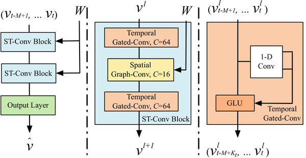
我们可以看到整个架构由三部分组成，原作者的图画得不够清晰。我放上我自己制作的图，如下所示。

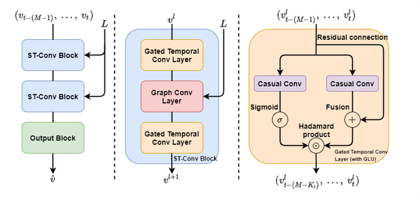
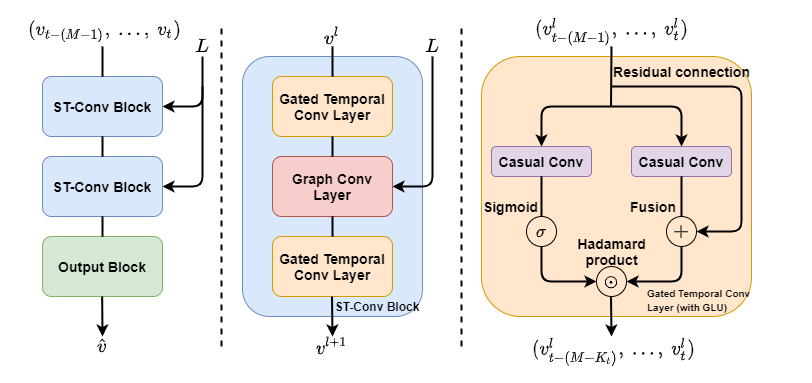
在论文中，我们可以知道，整个架构其實是「输入 —— ST-Conv Block —— ST-Conv Block —— Output Block —— 输出」。

1.1 ST-Conv Block

每一个 ST-Conv Block 是由两个 Gated Temporal Convolution layer 夹着一个 Graph Convolution layer 组成。之所以，TGC 的 channel number 是 64，SGC 的是 16，是因为原作者认为这种「三明治」结构既可以 achieve fast spatial-state propagation from graph convolution through temporal convolutions，又可以 helps the network sufficiently apply bottleneck strategy to achieve scale compression and feature squeezing by downscaling and upscaling of channels C through the graph convolutional layer.

2.1 Graph Convolution layer

从源代码来看，就是 Graph Convolution + Residual Connection。原作者采用了 ChebConv 和 GCNConv ，但是原作者对 GCNConv 的理解有误，论文中的公式和代码都写错了。

2.2 ChebConv（默认使用 \mathbf{L}_{\mathbb{norm}} = \mathbf{L}_{\mathbb{sym}} = \mathbf{D}^{-\frac{1}{2}}\mathbf{L}\mathbf{D}^{-\frac{1}{2}} =\mathbf{I}_{n} - \mathbf{D}^{-\frac{1}{2}}\mathbf{A}\mathbf{D}^{-\frac{1}{2}}，也可以使用 \mathbf{L}_{\mathbb{rw}} = \mathbf{D}_{row}^{-1}\mathbf{L} = \mathbf{I}_{n} - \mathbf{D}_{row}^{-1}\mathbf{A} ）

采用 Chebyshev polynomials of the first kind （第一类切比雪夫多项式）近似卷积核： g_{\theta}(\mathbf{\Lambda}) \approx \sum^{K-1}_{k=0}\theta_kT_k(\widetilde{\mathbf{\Lambda}}) ， \widetilde{\mathbf{\Lambda}} = \frac{2\mathbf{\Lambda}}{\lambda_{max}} - \mathbf{I}_{n} 。

其递推公式为 T_k(x) = 2xT_{k-1}(x) - T_{k-2}(x) ，其中 T_0(x) = 1 ， T_1(x) = x 。Graph convolution kernel size K_s 与 order of Chebyshev polynomials K_{cp} 不一致，因为前者是从 1 开始计数，而后者是从 0 开始计数。因此， K_s = K_{cp} + 1 。在公式和代码中，我用 K 代表 K_{s} ，注意 K \in [1,\ |\mathcal{V}|] 。

将卷积核公式代入原谱卷积公式中，得

\begin{split} g_{\theta}(\mathbf{L}_{\mathbb{norm}})\mathbf{x} &\approx \mathbf{U}\sum^{K-1}_{k=0}\theta_kT_k(\widetilde{\mathbf{\Lambda}})\mathbf{U}^T\mathbf{x} \\ &\approx \sum^{K-1}_{k=0}\theta_kT_k(\mathbf{U}\widetilde{\mathbf{\Lambda}}\mathbf{U}^T)\mathbf{x} \\ &\approx \sum^{K-1}_{k=0}\theta_kT_k(\widetilde{\mathbf{L}}_{\mathbb{norm}})\mathbf{x} \end{split}

其中 \widetilde{\mathbf{L}}_{\mathbb{norm}} = \frac{2\mathbf{L}_{\mathbb{norm}}}{\lambda_{max}} - \mathbf{I}_n 。为了使得时间复杂度从 O(n^2) 降至 O(K|\mathcal{E}|) ，ChebyNet 的作者提出用递推的写法，公式如下：

\bar{x}_{k} = 2\widetilde{\mathbf{L}}_{\mathbb{norm}}\bar{x}_{k-1} - \bar{x}_{k-2} ，其中 \bar{x}_{0} = x ， \bar{x}_{1} = \widetilde{\mathbf{L}}_{\mathbb{norm}}x 。

g_{\theta}(\mathbf{L}_{\mathbf{norm}})\mathbf{x} \approx [\bar{x}_{0},\ ...,\ \bar{x}_{K-1}]\mathbf{\Theta}

2.3 GCNConv

当我们把 ChebyNet 的图卷积公式中的 order K - 1 = 1 （即 K_{s} = 2 ）时，原式写作

g_{\theta}(\mathbf{L}_{\mathbb{norm}})\mathbf{x} \approx \mathbf{x}\mathbf{\Theta}_{0} + (\mathbf{L}_{norm}-\mathbf{I}_{n})\mathbf{x}\mathbf{\Theta}_{1} = \mathbf{x}\mathbf{\Theta}_{0} - (\mathbf{D}^{-\frac{1}{2}}\mathbf{A}\mathbf{D}^{-\frac{1}{2}})\mathbf{x}\mathbf{\Theta}_{1}

令 \mathbf{\Theta} = \mathbf{\Theta}_{0} = -\mathbf{\Theta}_{1} ，则原式化简为

g_{\theta}(\mathbf{L}_{\mathbb{norm}})\mathbf{x} \approx (\mathbf{I}_{n} + \mathbf{D}^{-\frac{1}{2}}\mathbf{A}\mathbf{D}^{-\frac{1}{2}})\mathbf{x}\mathbf{\Theta}

因为 \mathbf{I}_{n} + \mathbf{D}^{-\frac{1}{2}}\mathbf{A}\mathbf{D}^{-\frac{1}{2}} 的特征值 \in [0,\ 2] ，为防止梯度消失（梯度弥散）或梯度爆炸（这是写在 paper 中的说辞，实际原因是此为 high-pass filter），采用 renormalization trick（重归一化技巧），即

\mathbf{I}_{n} + \mathbf{D}^{-\frac{1}{2}}\mathbf{A}\mathbf{D}^{-\frac{1}{2}} \rightarrow \widetilde{\mathbf{D}}^{-\frac{1}{2}}\widetilde{\mathbf{A}} \widetilde{\mathbf{D}}^{-\frac{1}{2}} ，其中 \widetilde{\mathbf{A}} = \mathbf{A} + \mathbf{I}_{n} ， \widetilde{\mathbf{D}}_{ii} = \sum_{j} \widetilde{\mathbf{A}}_{ij} 。

所以，原图卷积公式可以进一步近似为

g_{\theta}(\mathbf{L}_{\mathbb{norm}})\mathbf{x} \approx g_{\theta}(\hat{\mathbf{A}})\mathbf{x} = \hat{\mathbf{A}}\mathbf{x}\mathbf{\Theta} ，其中 \hat{\mathbf{A}} = \widetilde{\mathbf{D}}^{-\frac{1}{2}}\widetilde{\mathbf{A}}\widetilde{\mathbf{D}}^{-\frac{1}{2}} 。

每层图卷积的时间复杂度为 O(|\mathcal{E}|) 。

3.1 Temporal Gated Convolution layer

Temporal Gated Convolution layer 是由 Casual Convolution 和 Gated Linear Unit (GLU) 组合而成。

与典型的 GLU 不同的是，其中的 1D Convolution 被 Casual Convolution 所取代，最后的 convolution 被 Hadamard Product 所取代。原论文中提到的 Residual Connection ，并不接在 Hadamard Product 之后，而是与 Casual Convolution 之后产生 P 的那一段相连，使得原始输入与 P 融合。

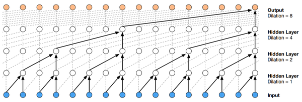
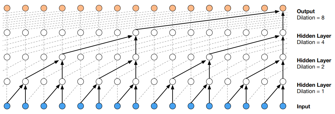
3.2 Casual Convolution 和 Dilated (Casual) Convolution

Casual convolution: convolutions where an output at time t is convolved only with elements from time t and earlier in the previous layer.

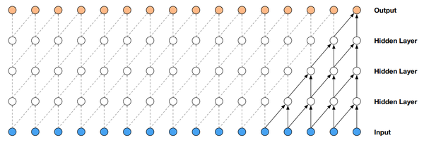
Dilated (casual) convolution 定义为 F(s) = (\textbf x *_{d} f)(s) = \sum^{k-1}_{i=0}f(i) \cdot \textbf x_{s-d \cdot i}

3.3 Gated Linear Unit (GLU) 和 Gated Tanh Unit (GTU)

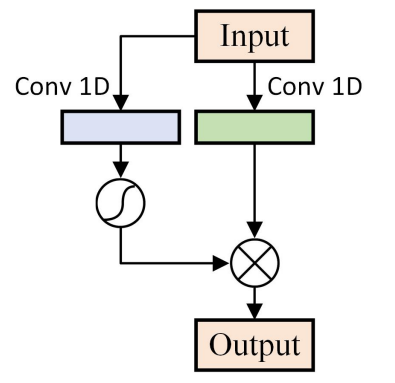
Gated linear unit (GLU): 将输入序列分成两部分，分别经过 1D-conv，之后，一部分经过 Sigmoid，另一部分直出，然后两者经过一次 convolution，最后输出。公式如下： h_{l}(X) = (X * W + b) \otimes \sigma(X * V + c)

PyTorch 团队提出，其实作应为 \mathbf{X}_{a}\odot\sigma(\mathbf{X}_{b})

Gated Tanh unit (GTU): 类似于 GLU，GLU 中线性的部分换为 Tanh。公式如下:

h_{l}(X) = tanh(X * W + b) \otimes \sigma(X * V + c)

有人认为，应实作为 \tanh(\mathbf{X}_{a}) \odot \sigma(\mathbf{X}_{b})

4.1 weighted adjacency matrix

STGCN 的作者并没有理解 GNN（从他把 GCN 当作是 1^{st} order ChebyNet 就可以看出来 ），把计算「带权重的邻接矩阵」的公式搞错了，我强烈建议你采用 ChebyNet 所提供的计算公式。公式如下：

w_{ij}=\left\{ \begin{aligned} \exp(-\frac{{[\mathbb{dist}(v_i,\ v_j)]}^2}{\sigma^2}), && \mathbb{if} \ \mathbb{dist}(v_i, v_j)\le k \\ 0, && \mathbb{otherwise} \end{aligned} \right.

二、代码解析

1.1 model 整体架构

由于原 paper 所写 model 有两个，分别是用 ChebNet 和 GCN 的 Graph Convolution 的 STGCN，原作者定义为 STGCN(Cheb) 和 STGCN( 1^{st} )，我在代码中定义为 STGCN(ChebGraphConv) 和 STGCN(GraphConv)。

Causal Convolution

class CausalConv1d(nn.Conv1d):
    def __init__(self, in_channels, out_channels, kernel_size, stride=1, enable_padding=False, dilation=1, groups=1, bias=True):
        if enable_padding == True:
            self.__padding = (kernel_size - 1) * dilation
        else:
            self.__padding = 0
        super(CausalConv1d, self).__init__(in_channels, out_channels, kernel_size=kernel_size, stride=stride, padding=self.__padding, dilation=dilation, groups=groups, bias=bias)

    def forward(self, input):
        result = super(CausalConv1d, self).forward(input)
        if self.__padding != 0:
            return result[: , : , : -self.__padding]
        
        return result

class CausalConv2d(nn.Conv2d):
    def __init__(self, in_channels, out_channels, kernel_size, stride=1, enable_padding=False, dilation=1, groups=1, bias=True):
        kernel_size = nn.modules.utils._pair(kernel_size)
        stride = nn.modules.utils._pair(stride)
        dilation = nn.modules.utils._pair(dilation)
        if enable_padding == True:
            self.__padding = [int((kernel_size[i] - 1) * dilation[i]) for i in range(len(kernel_size))]
        else:
            self.__padding = 0
        self.left_padding = nn.modules.utils._pair(self.__padding)
        super(CausalConv2d, self).__init__(in_channels, out_channels, kernel_size, stride=stride, padding=0, dilation=dilation, groups=groups, bias=bias)
        
    def forward(self, input):
        if self.__padding != 0:
            input = F.pad(input, (self.left_padding[1], 0, self.left_padding[0], 0))
        result = super(CausalConv2d, self).forward(input)

        return result

Cheby Graph Convolution

class ChebGraphConv(nn.Module):
    def __init__(self, c_in, c_out, Ks, gso, bias):
        super(ChebGraphConv, self).__init__()
        self.c_in = c_in
        self.c_out = c_out
        self.Ks = Ks
        self.gso = gso
        self.weight = nn.Parameter(torch.FloatTensor(Ks, c_in, c_out))
        if bias:
            self.bias = nn.Parameter(torch.FloatTensor(c_out))
        else:
            self.register_parameter('bias', None)
        self.reset_parameters()

    def reset_parameters(self):
        init.kaiming_uniform_(self.weight, a=math.sqrt(5))
        if self.bias is not None:
            fan_in, _ = init._calculate_fan_in_and_fan_out(self.weight)
            bound = 1 / math.sqrt(fan_in) if fan_in > 0 else 0
            init.uniform_(self.bias, -bound, bound)
    
    def forward(self, x):
        #bs, c_in, ts, n_vertex = x.shape
        x = torch.permute(x, (0, 2, 3, 1))

        if self.Ks - 1 < 0:
            raise ValueError(f'ERROR: the graph convolution kernel size Ks has to be a positive integer, but received {self.Ks}.')  
        elif self.Ks - 1 == 0:
            x_0 = x
            x_list = [x_0]
        elif self.Ks - 1 == 1:
            x_0 = x
            x_1 = torch.einsum('hi,btij->bthj', self.gso, x)
            x_list = [x_0, x_1]
        elif self.Ks - 1 >= 2:
            x_0 = x
            x_1 = torch.einsum('hi,btij->bthj', self.gso, x)
            x_list = [x_0, x_1]
            for k in range(2, self.Ks):
                x_list.append(torch.einsum('hi,btij->bthj', 2 * self.gso, x_list[k - 1]) - x_list[k - 2])
        
        x = torch.stack(x_list, dim=2)

        cheb_graph_conv = torch.einsum('btkhi,kij->bthj', x, self.weight)

        if self.bias is not None:
            cheb_graph_conv = torch.add(cheb_graph_conv, self.bias)
        else:
            cheb_graph_conv = cheb_graph_conv
        
        return cheb_graph_conv

Graph Convolution

class GraphConv(nn.Module):
    def __init__(self, c_in, c_out, gso, bias):
        super(GraphConv, self).__init__()
        self.c_in = c_in
        self.c_out = c_out
        self.gso = gso
        self.weight = nn.Parameter(torch.FloatTensor(c_in, c_out))
        if bias:
            self.bias = nn.Parameter(torch.FloatTensor(c_out))
        else:
            self.register_parameter('bias', None)
        self.reset_parameters()

    def reset_parameters(self):
        init.kaiming_uniform_(self.weight, a=math.sqrt(5))
        if self.bias is not None:
            fan_in, _ = init._calculate_fan_in_and_fan_out(self.weight)
            bound = 1 / math.sqrt(fan_in) if fan_in > 0 else 0
            init.uniform_(self.bias, -bound, bound)

    def forward(self, x):
        #bs, c_in, ts, n_vertex = x.shape
        x = torch.permute(x, (0, 2, 3, 1))

        first_mul = torch.einsum('hi,btij->bthj', self.gso, x)
        second_mul = torch.einsum('bthi,ij->bthj', first_mul, self.weight)

        if self.bias is not None:
            graph_conv = torch.add(second_mul, self.bias)
        else:
            graph_conv = second_mul
        
        return graph_conv

更多的代码与细节，欢迎关注我的 GitHub repository：hazdzz/STGCN ，为了照顾大陆用户，奉上码云（Gitee）的项目链接：hazdzz/STGCN 。