R_ggplot2基础(一)

作者:李誉辉 四川大学在读研究生
往期精彩:
1 ggplot2特点
采用图层的设计方式,有利于结构化思维
将表征数据和图形细节分开,能快速将图形表现出来,使创造性绘图更加容易,而不必纠结于图形的细节,细节可以后期慢慢调整
将常见的统计变换融入到了绘图中
有明确的起始(ggplot开始)与终止(一句话一个图层),图层之间的叠加是靠“+”实现的,越往后,其图层越在上方
图形美观,扩展包丰富,有专门调整字体和公式的包,有专门调整颜色的包,还有专门用按钮辅助调整主题的包,总之,应有尽有
2 ggplot2基本概念
Data数据, Mapping映射
Scale标度
Geometric几何对象
Statistics统计变换
Coordinate坐标系统
Layer图层
Facet分面
Legend图例
beautiful美化
3 ggplot2语法框架
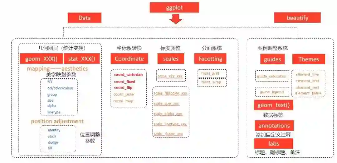
绘图流程:
ggplot(data, aes(x = , y = )) +   # 基础图层,不出现任何图形元素,
  geom_xxx()|stat_xxx() +  # 几何图层或统计变换,出现图形元素
  coord_xxx() +  # 坐标变换,默认笛卡尔坐标系
  scale_xxx() + # 标度调整,调整具体的标度
  facet_xxx() + # 分面,将其中一个变量进行分面变换
  guides() + # 图例调整
  theme() # 主题系统
3.1 共性映射与个性映射
ggplot(data = NULL, mapping = aes())geom_xxx(data = NULL, mapping = aes())ggplot()内有data、mapping两个参数
具有全局优先级,可以被之后的所有geom_xxx对象或stat_xxx()所继承(前提是geom或stat未指定相关参数)而
geom_xxx()或stat_xxx()内的参数属于局部参数,仅仅作用于内部为了避免混乱,通常将共性映射的参数指定在
ggplot(aes())aes内部,将个性映射的参数指定在geom_xxx(aes())或stat_xxx(aes())内部
3.2 几何对象与统计变换
几何对象
geom_xxx(stat = )内有统计变换参数stat,统计变换stat_xxx(geom = )内也有几何对象参数geom两种方法结果相同,几何对象更专注于结果,统计变换更专注于变换过程
library(ggplot2)
# 用几何对象作图
ggplot(data = NULL, mapping = aes(x = x, y = y)) + geom_point(color = "darked",
    stat = "identity")  # identity 表示没有任何统计变换
# 用统计变换作图
ggplot(data = NULL, mapping = aes(x = x, y = y)) + stat_identity(color = "darked",
    geom = "point")  # geom_point(stat = 'identity')与stat_identity(geom = 'point')结果一样
3.3 aes与data参数
aes参数用来指定要映射的变量,可以是多个变量,
data参数表示指定数据源,必须是data.frame格式,其坐标轴变量最好宽转长,只能指定一个x轴和y轴,多个x列或y列不能使用调整图例。
4 geom_xxx()几何对象
常用的几种几何对象函数:
| 几何对象函数 | 描述 | 其它 |
|---|---|---|
geom_point |
点图 | geom_point(position = "jitter") == geom_jitter() 避免重叠 |
geom_line |
折线图 | 可以通过smooth参数平滑处理 |
geom_bar |
柱形图 | x轴是离散变量 |
geom_area |
面积图 | |
geom_histogram |
直方图 | x轴数据是连续的 |
geom_boxplot |
箱线图 | |
geom_rect |
二维长方形图 | |
geom_segment |
线段图 | |
geom_path |
几何路径 | 由一组点按顺序连接 |
geom_curve |
曲线 | |
geom_abline |
斜线 | 有斜率和截距指定 |
geom_hline |
水平线 | 常用于坐标轴绘制 |
geom_vline |
竖线 | 常用于坐标轴绘制 |
geom_text |
文本 |
ggplot2唯一不支持的常规平面图形是雷达图
其它几何对象查询:
ggplot2 part of the tidyverse
ggplot2 Quick Reference: geom
也可以用
ls(pattern = '^geom_', env = as.environment('package:ggplot2')) 查询,但是没有图形示例
library(ggplot2)
ls(pattern = "^geom_", env = as.environment("package:ggplot2"))
柱形图和散点图是关键,并且与极坐标变换紧密相连,着重介绍柱形图和散点图,其它的原理和参数都类似
4.1 aesthetics specifications 美学参数
能用作变量映射的包括:
| 美学参数 | 描述 |
|---|---|
| color/col/colour | 指定点、线和填充区域边界的颜色 |
| fill | 指定填充区域的颜色,如条形和密度区域, 第21到24号点也有填充色 |
| alpha | 指定颜色的透明度,从0(完全透明) 到 1(不透明) |
| size | 指定点的尺寸或线的宽度,单位为mm |
| angle | 角度,只有部分几何对象有,如geom_text文本的摆放角度, geom_spoke中短棒摆放角度 |
| linetype | 指定线条的类型 |
| shape | 点的形状, 为[0, 25]区间的26个整数 |
| vjust | 垂直位置微调,在(0, 1)区间的数字或位置字符串: 0=“buttom”, 0.5=“middle”, 1=“top” , 区间外的数字微调比例控制不均 |
| hjust | 水平位置微调,在(0, 1)区间的数字或位置字符串:0=“left”, 0.5=“center”, 1=“right” , 区间外的数字微调比例控制不均 |
| 不常映射的参数 | 描述 |
|---|---|
| binwidth | 直方图的宽度 |
| notch | 表示方块图是否应为缺口 |
| sides | 表示地毯图的安置位置(“b”底部, “l”左部, “t”顶部, “r”右部, “bl”左下角, 等等) |
| width | 箱线图或柱形图的宽度,从(0, 1), 柱形图默认0.9即90% |
| lineend | 表示指定宽线条端部形状,有3种:“round”半圆形,“square”增加方形, “butt”默认不变, 常用于geom_path和geom_line几何对象 |
| family | 字体(Font face),内置的只有3种:“sans”, “serif”, “mono” |
| fontface | 字型,分为: “plain”常规体, “bold”粗体, “italic”斜体, “bold.italic”粗斜体。常用于geom_text等文本对象 |
| lineheight | 长文本换行行距, 常用于geom_text等文本对象 |
4.1.1 fill/color 颜色
R自身自持很多种方式的颜色,“颜色名称”和“HEX色值”最常用和方便,其它的需要扩展包
颜色名称如:
“white”, “azure”, “bisque”, “blue”, “black”, “brown”, “chacolate”, “coral”, “cornsilk”, “cyan”, “gold” ,
“darkgolden”, “orange”, “orchild”, “gray”, “grey”, “tomato”, “violet”, “wheat”, “yellow”, “pink”,
“purple”, “red”, “salmon”, “seashell”, “ivory”,“magentia”,“navy”等系列。
所有的颜色名称见: R_Color_Chart(后台回复:颜色,可下载PDF版本)
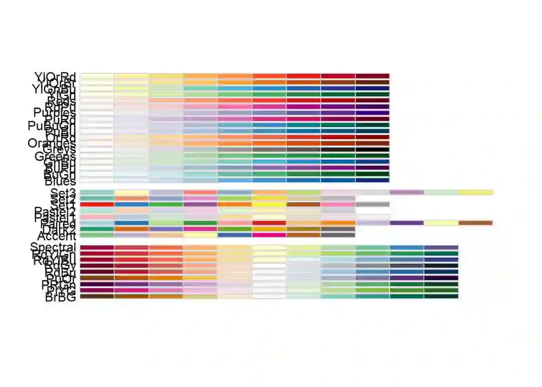
如果对一组颜色进行映射的话,建议使用RColorBrewer等调色包,更加方便
RColorBrewer颜色板如下,左边为字符串编号,上下分为3个版块,分别为渐变色板Sequential,离散对比色板Qualitative,两极色板Diverging
# colors() # 调用所有内置颜色编号,名称
scales::show_col(colors()[1:6])  # show_col函数可以将颜色名称或HEX色值向量显示出来
# RColorBrewer包使用
library("RColorBrewer")
display.brewer.all()  # 显示所有可用色板
display.brewer.all(type = "seq")  # 查看渐变色板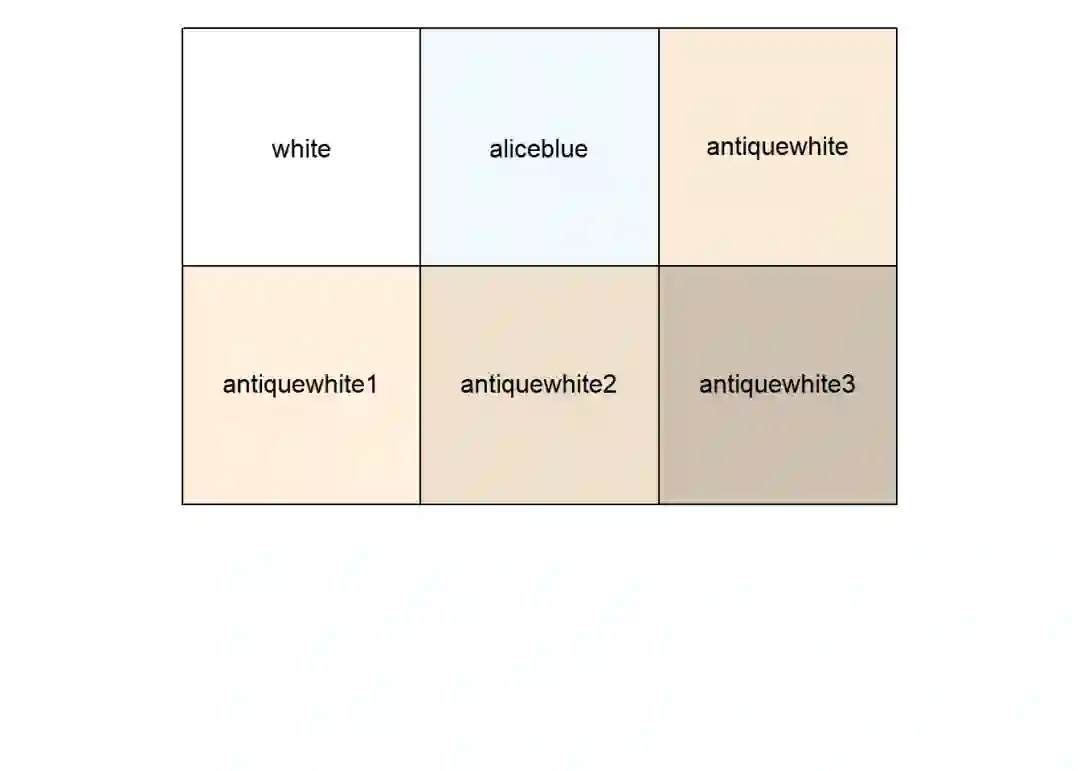
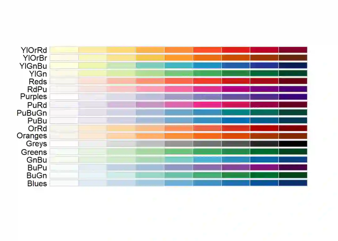
RColorBrewer使用方法:
通过函数brewer.pal(n, name)抽取色条名字为name的n种颜色,后面还可以用“[]”索引符号索取色块,
一个几何对象设置多种颜色只能在标度中设置,我们会在标度中继续讲解,例:
library("RColorBrewer")
display.brewer.pal(7, "PuRd")  # 抽取PuRd色条7种颜色,其颜色色值范围没有变,只是色值间隔增大了
display.brewer.pal(9, "PuRd")[11]  # 抽取PuRd色条11种颜色,其颜色色值范围没有变,指定色值间隔减小了
4.1.2 linetype 线型
线条形状通过名称或整数指定:
| 线型 | 描述 |
|---|---|
| 0=“blank” | 白线 |
| 1=“solid” | 实线 |
| 2=“dashed” | 短虚线 |
| 3=“dotted” | 点线 |
| 4=“dotdash” | 点横线 |
| 5=“longdash” | 长虚线 |
| 6=“twodash” | 短长虚线 |
自定义线型
通过1个十六进制的字符串来自定义,字符串长度为2、4、6或8。
第1个数字为代表闭合的长度,第2个数字代表缺口的长度,第3个数字又是闭合的长度,第4个数字是缺口的长度,如此交替排列。 然后作为一个整体重复排列
如:
* 字符串“33”代表开始3个单位长度闭合,产生短横线,然后缺口长度也是3个单位,这样作为一个整体进行重复排列
* 字符串“81”代表开始8个单位长度闭合,产生较长的横线,然后缺口长度为1个单位,这样作为一个整体重复排列
* 字符串“f8”表示开始16个单位长度闭合,产生长横线,然后缺口长度为8个单位,这样作为一个整体重复排列
* 字符串“357a”表示开始3个单位长度闭合,产生短横线,然后缺口5个单位,然后闭合7个单位,最后缺口11个单位,这样整体重复排列
如图所示:
library(ggplot2)
lty <- c("solid", "dashed", "dotted", "dotdash", "longdash", "twodash")
linetypes <- data.frame(
  y = seq_along(lty), # seq_along表示生成与对象同样长度的序列
  lty = lty
)
ggplot(linetypes, aes(0, y)) +
  geom_segment(aes(xend = 5, yend = y, linetype = lty)) +  # 将一个变量映射到线型
  scale_linetype_identity() +
  geom_text(aes(label = lty), hjust = 0, nudge_y = 0.2) +
  scale_x_continuous(NULL, breaks = NULL) +
  scale_y_reverse(NULL, breaks = NULL)

# 自定义线型
lty <- c("33", "18", "81", "f8", "5f", "357a", "5a73", "342167", "a23f45b6") # 自定义9种线型
linetypes <- data.frame(
  y = seq_along(lty),
  lty = lty
)
ggplot(linetypes, aes(0, y)) +
  geom_segment(aes(xend = 5, yend = y, linetype = lty)) + # 将一个变量映射到线型
  scale_linetype_identity() +
  geom_text(aes(label = lty), hjust = 0, nudge_y = 0.2) +
  scale_x_continuous(NULL, breaks = NULL) +
  scale_y_reverse(NULL, breaks = NULL)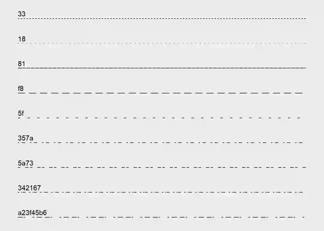
4.1.3 shape点型
[0, 25]个序号代表26种点型, 只有21到26号点形能fill颜色,其它都只有轮廓颜色,
序号32:127对应ASCII字符
所有序号如图所示:
library("ggplot2")

d = data.frame(p = c(0:25, 32:127))
ggplot() + scale_y_continuous(name = "") + scale_x_continuous(name = "") + scale_shape_identity() +
    geom_point(data = d, mapping = aes(x = p%%16, y = p%/%16, shape = p), size = 5,
        fill = "red") + geom_text(data = d, mapping = aes(x = p%%16, y = p%/%16 +
    0.25, label = p), size = 3)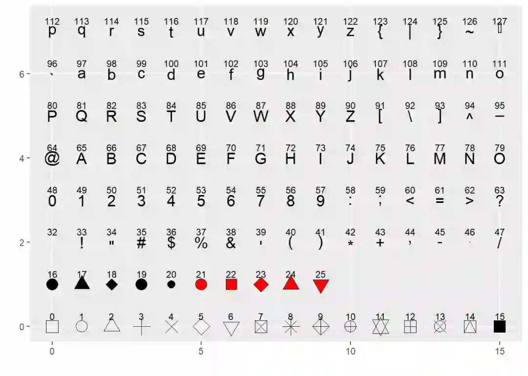
4.1.4 family字体
内置的只有3种,可以通过扩展包extrafont来将其它字体转换为ggplot2可识别的标准形式 还可以通过showtext包以图片的形式将字体插入到ggplot2图中,对于公式之类的特殊字体特别方便,比Latex容易爆了
library("ggplot2")

df <- data.frame(x = c(0.4, 0.6, 0.8), y = 1:3, family = c("sans", "serif",
    "mono"))
ggplot(df, aes(x, y)) + geom_text(aes(label = family, family = family), size = 15) +
    xlim(0.2, 1) + ylim(0, 4)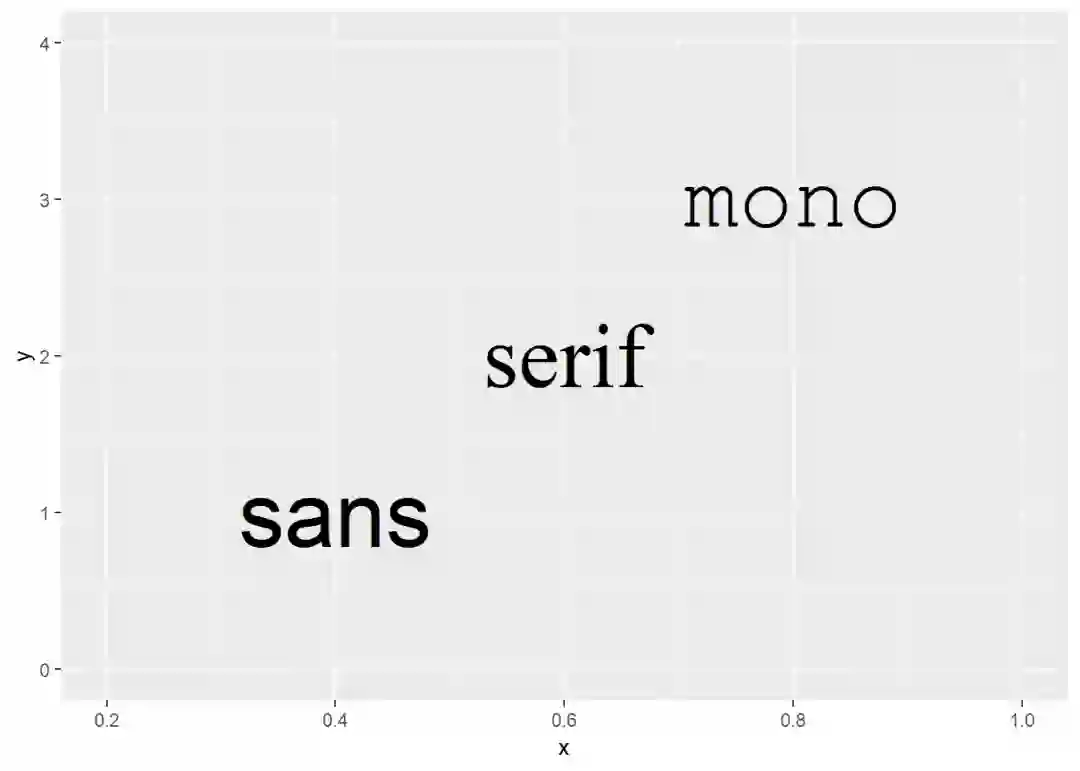
4.1.5 Font face字型
分为4类:“plain”常规体, “bold”粗体, “italic”斜体, “bold.italic”粗斜体
library("ggplot2")

df <- data.frame(x = c(1, 1.5, 3, 3.5), y = c(2, 1, 1, 2), fontface = c("plain",
    "bold", "italic", "bold.italic"))
ggplot(df, aes(x, y)) + geom_text(aes(label = fontface, fontface = fontface),
    size = 15) + xlim(0, 5.5) + ylim(0.5, 2.5)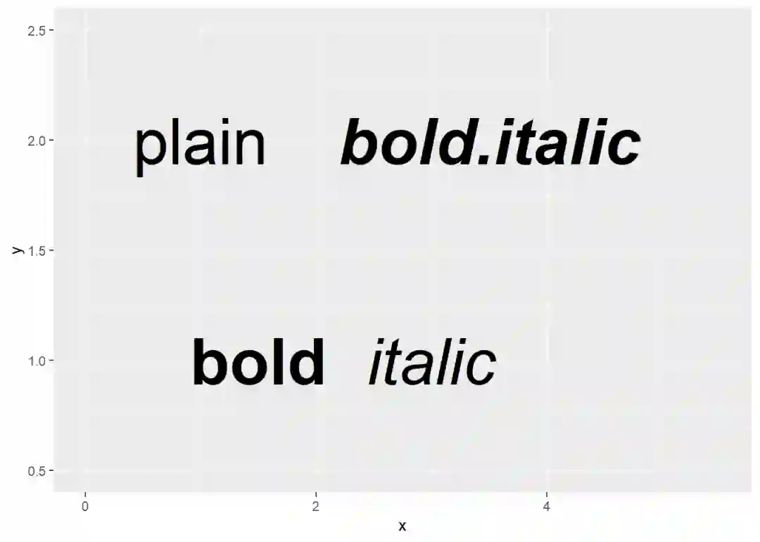
4.1.6 vjust/hjust相对位置微调
vjust: “top” = 1, “middle” = 0.5, “bottom” = 0
hjust: “left” = 0, “center” = 0.5, “right” = 1
微调后,该几何对象还是在另一个几何对象周围
library("ggplot2")

just <- expand.grid(hjust = c(0, 0.5, 1), vjust = c(0, 0.5, 1))
just$label <- paste0(just$hjust, ", ", just$vjust)

ggplot(just, aes(hjust, vjust)) + geom_point(colour = "grey70", size = 5) +
    geom_text(aes(label = label, hjust = hjust, vjust = vjust))  # 也能进行映射,但很少用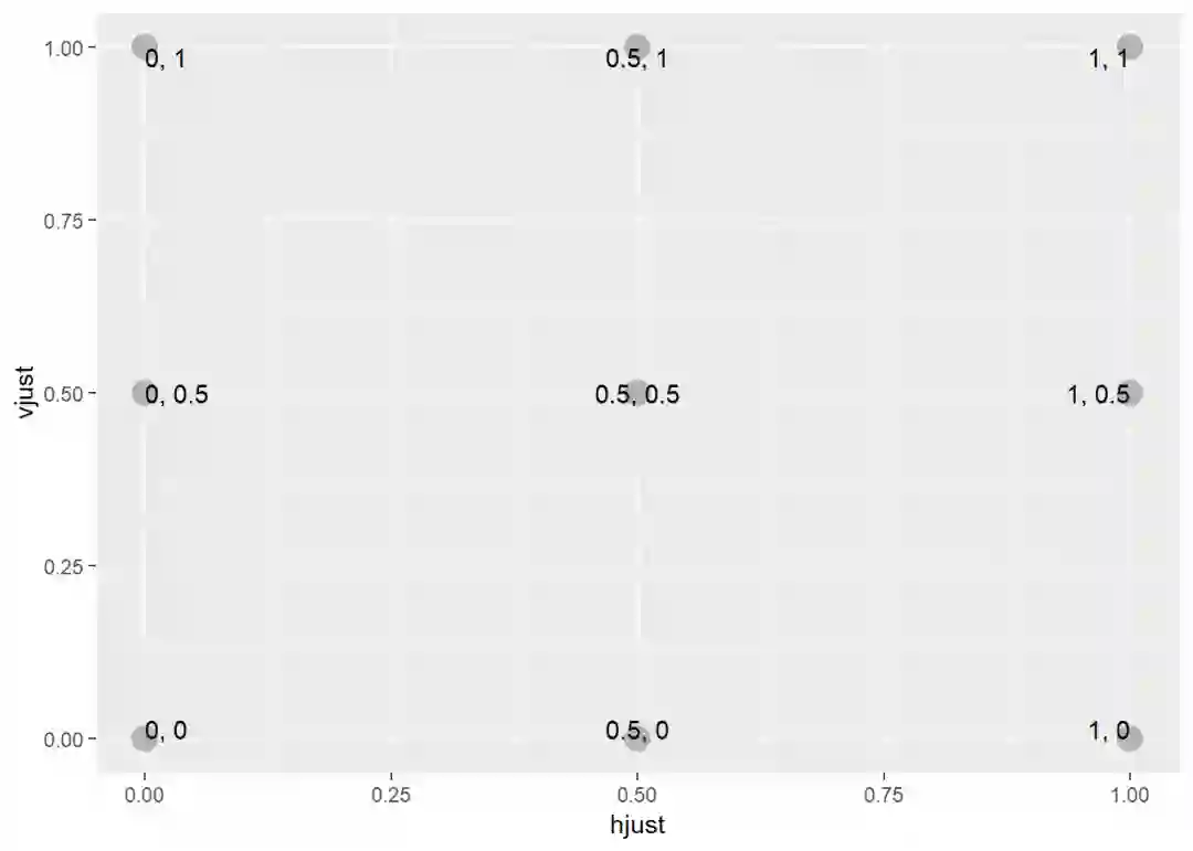
4.2 position adjustment 位置调整参数
包括:
| 位置调整函数 | 描述 | 其它 |
|---|---|---|
| position_dodge() | 水平并列放置 | position_dodge(width = NULL, preserve = c(“total”, “single”)) 簇状柱形图 |
| position_dodge2() | 水平并列放置 | position_dodge2(…, padding = 0.1, reverse = FALSE) 簇状柱形图,多了2个参数 |
| position_identity() | 位置不变 | 对于散点图和折线图,可行,默认为identity,但对于多分类柱形图,序列间存在遮盖 |
| position_stack() | 垂直堆叠 | position_stack(vjust = 1, reverse = FALSE) 柱形图和面积图默认stack堆积 |
| position_fill() | 百分比填充 | position_fill(vjust = 1, reverse = FALSE) 垂直堆叠,但只能反映各组百分比 |
| position_jitter() | 扰动处理 | position_jitter(width = NULL, height = NULL, seed = NA)部分重叠, 用于点图 |
| position_jitterdodge() | 并列抖动 | position_jitterdodge(jitter.width = NULL,jitter.height = 0, dodge.width = 0.75,seed = NA) |
| position_nudge() | 整体位置微调 | position_nudge(x = 0, y = 0),整体向x和y方向平移的距离,常用于geom_text文本对象 |
position_xxx()内其它参数:padding, preserve, reverse, vjust, width, height 等
| 参数名称 | 值 | 描述 |
|---|---|---|
| preserve | c(“total”, “single”) | 当同一组柱子高度相同时,是保留单个柱子,还是保留所有柱子 |
| padding | 数字,(0, 1)区间 | 调整柱子间距(中心距离), 越大,则柱子宽度缩小越多, 间距越大,0.5表示宽度缩小50%以增大间距 |
| reverse | TRUE/FALSE | 是否翻转各组柱子内部的排列顺序,对于dodge2则水平顺序翻转,对于stack和fill则垂直顺序不同 |
| vjust | (0,1)区间 | 调整点和线的垂直位置,默认1顶部,0.5表示居中,0表示处于底部,折线的变化趋势会变平缓,默认1 |
| width | (0,1)区间 | 表示水平抖动的程度,因为存在正负方向,所有抖动的范围为其2倍,默认0.5 |
| height | (0,1)区间 | 表示垂直抖动的程度,因为存在正负方向,所以抖动的范围为其2倍, 默认0.5 |
| dodge.width | (0,1)区间 | 表示各组的点抖动总的水平宽度,默认0.75, 表示点分布在各组箱子75%宽度上 |
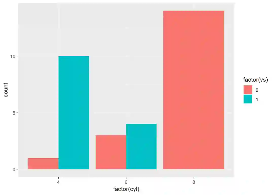
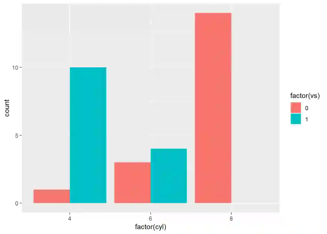
4.2.1 position_dodge(), position_dodge2() 水平并列
library(ggplot2)
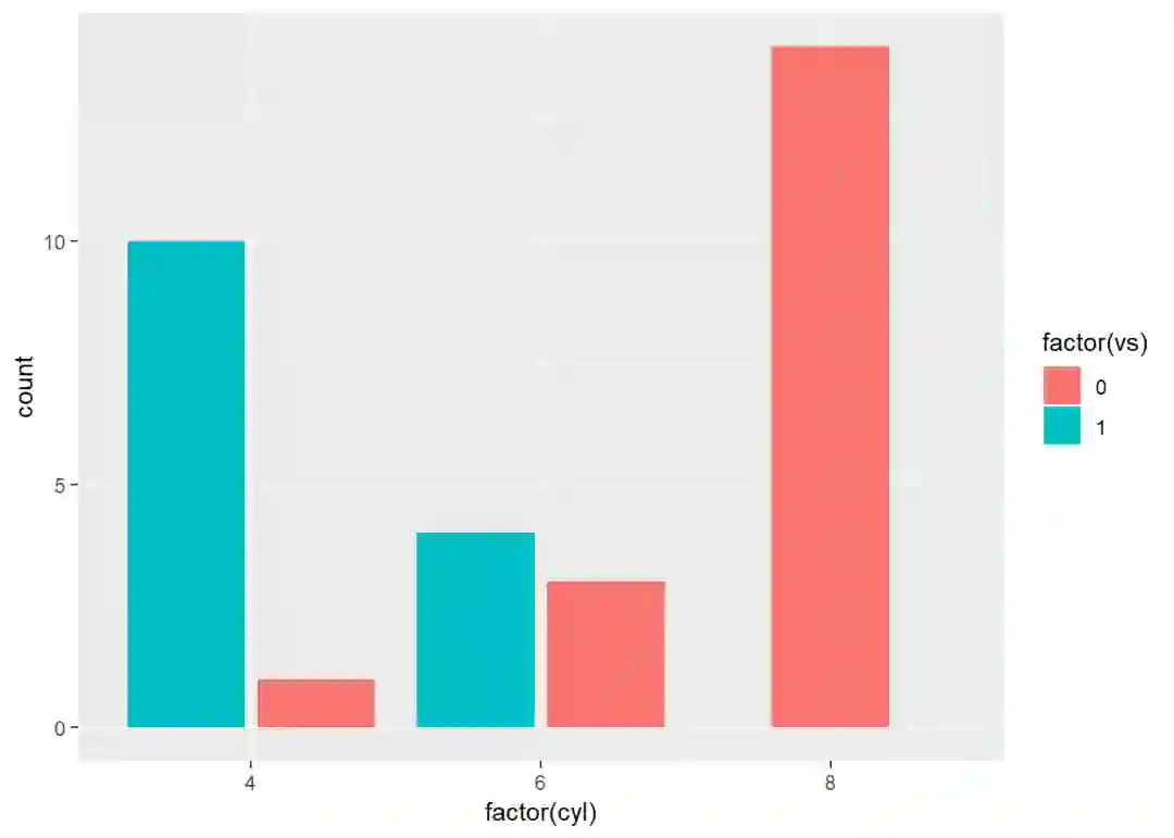
ggplot(mtcars, aes(factor(cyl), fill = factor(vs))) + geom_bar(position = "dodge2") # 水平并列柱形图,默认保留所有柱子
ggplot(mtcars, aes(factor(cyl), fill = factor(vs))) + geom_bar(position = position_dodge(preserve = "total")) # 保留所有柱子
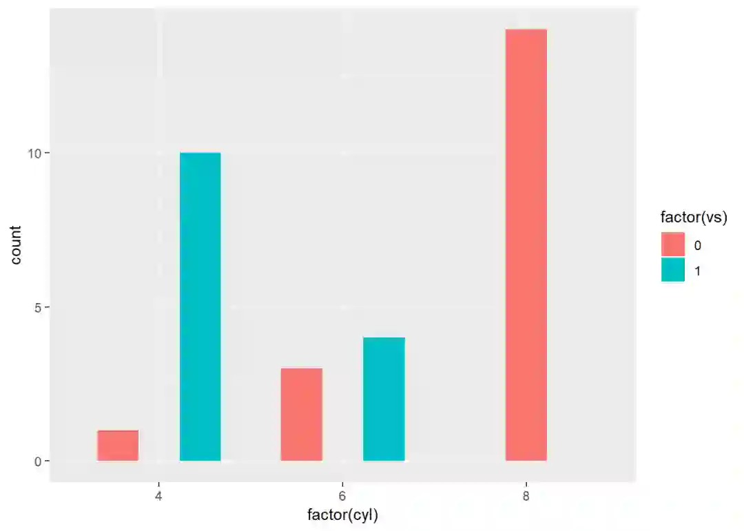
ggplot(mtcars, aes(factor(cyl), fill = factor(vs))) + geom_bar(position = position_dodge(preserve = "single")) # 保留单个柱子
ggplot(mtcars, aes(factor(cyl), fill = factor(vs))) + geom_bar(position = position_dodge2(preserve = "single",
reverse = T)) # 翻转各组柱子内部排列顺序
ggplot(mtcars, aes(factor(cyl), fill = factor(vs))) + geom_bar(position = position_dodge2(preserve = "single",
padding = 0.5)) # 所有柱子宽度缩小50%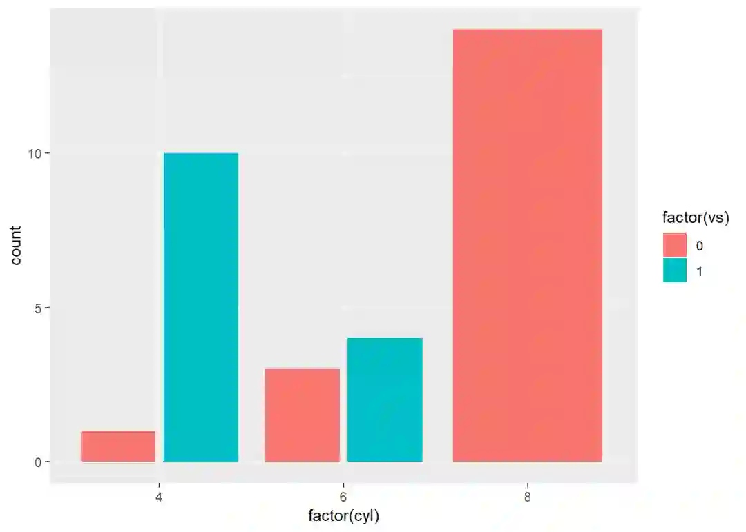
4.2.2 position_stack, position_fill 垂直堆积
library(ggplot2)
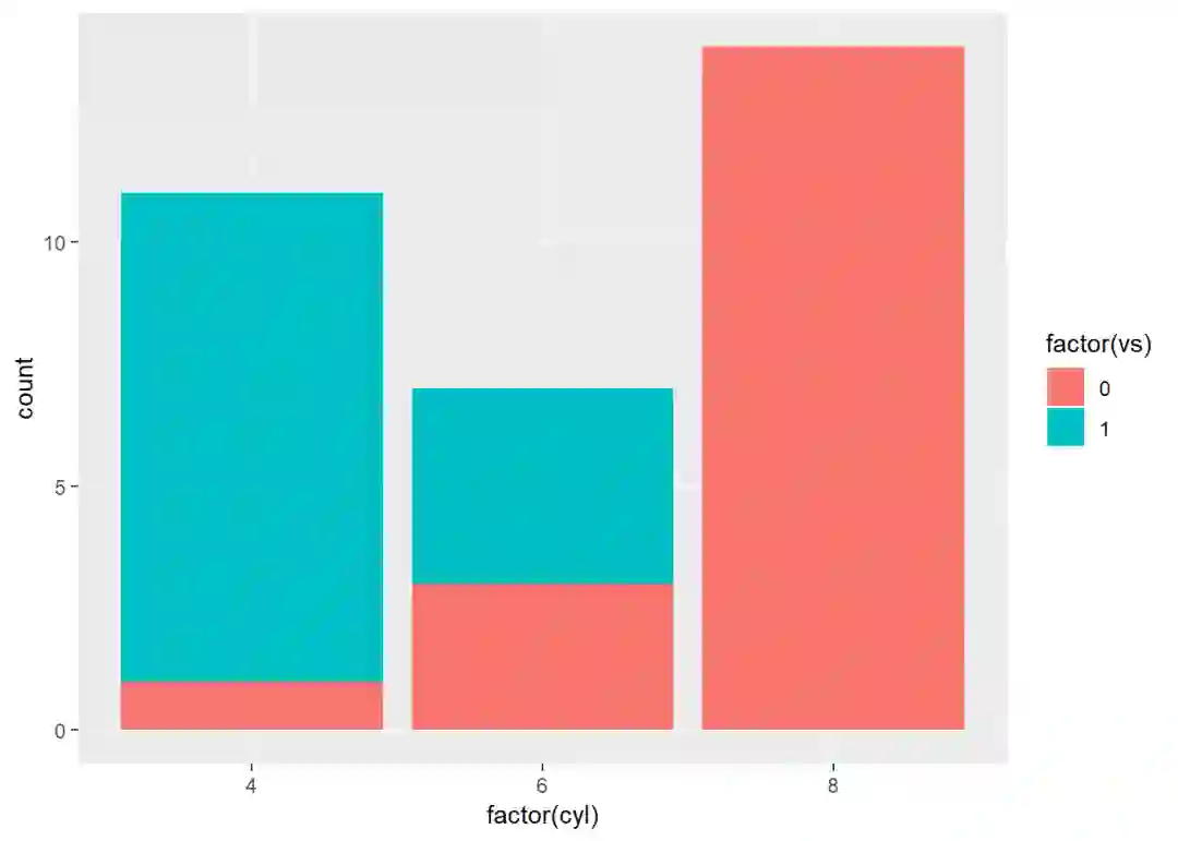
ggplot(mtcars, aes(factor(cyl), fill = factor(vs))) + geom_bar() # 柱形图默认stack堆积
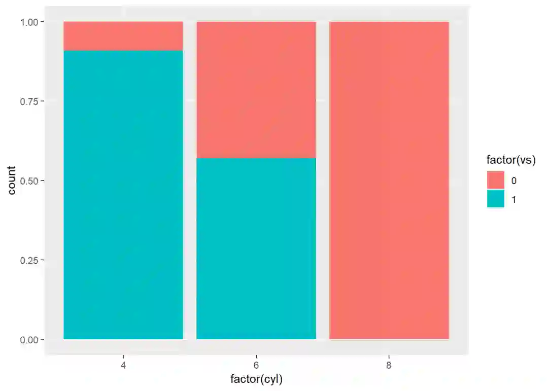
ggplot(mtcars, aes(factor(cyl), fill = factor(vs))) + geom_bar(position = "fill") # 百分比堆积
ggplot(mtcars, aes(factor(cyl), fill = factor(vs))) + geom_bar(position = position_stack(reverse = TRUE)) # 翻转各组内部垂直堆叠顺序
# 散点图 + 折线图
series <- data.frame(time = c(rep(1, 4), rep(2, 4), rep(3, 4), rep(4, 4)), type = rep(c("a",
"b", "c", "d"), 4), value = rpois(16, 10))
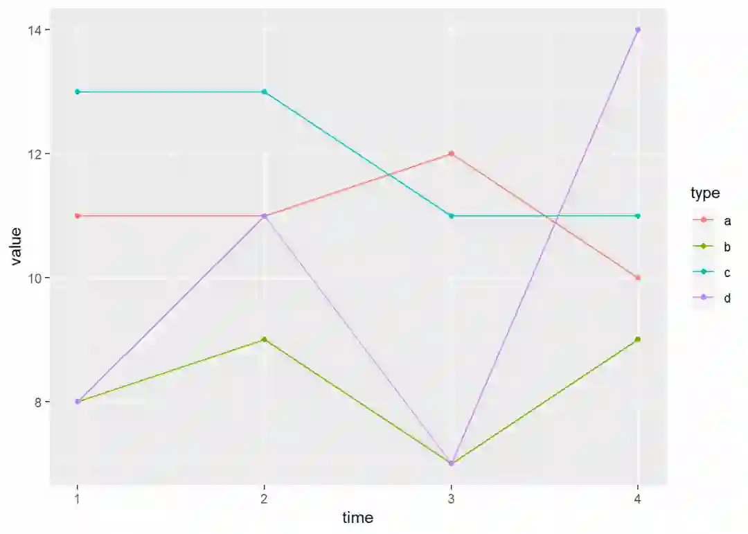
ggplot(series, aes(time, value, group = type)) + geom_line(aes(colour = type)) +
geom_point(aes(colour = type)) # 默认identity
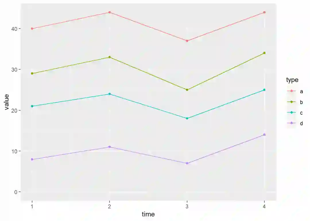
ggplot(series, aes(time, value, group = type)) + geom_line(aes(colour = type),
position = "stack") + geom_point(aes(colour = type), position = "stack") # stack堆积
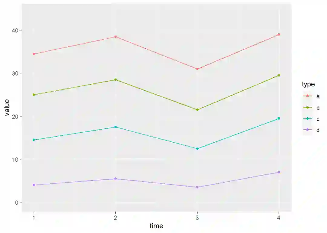
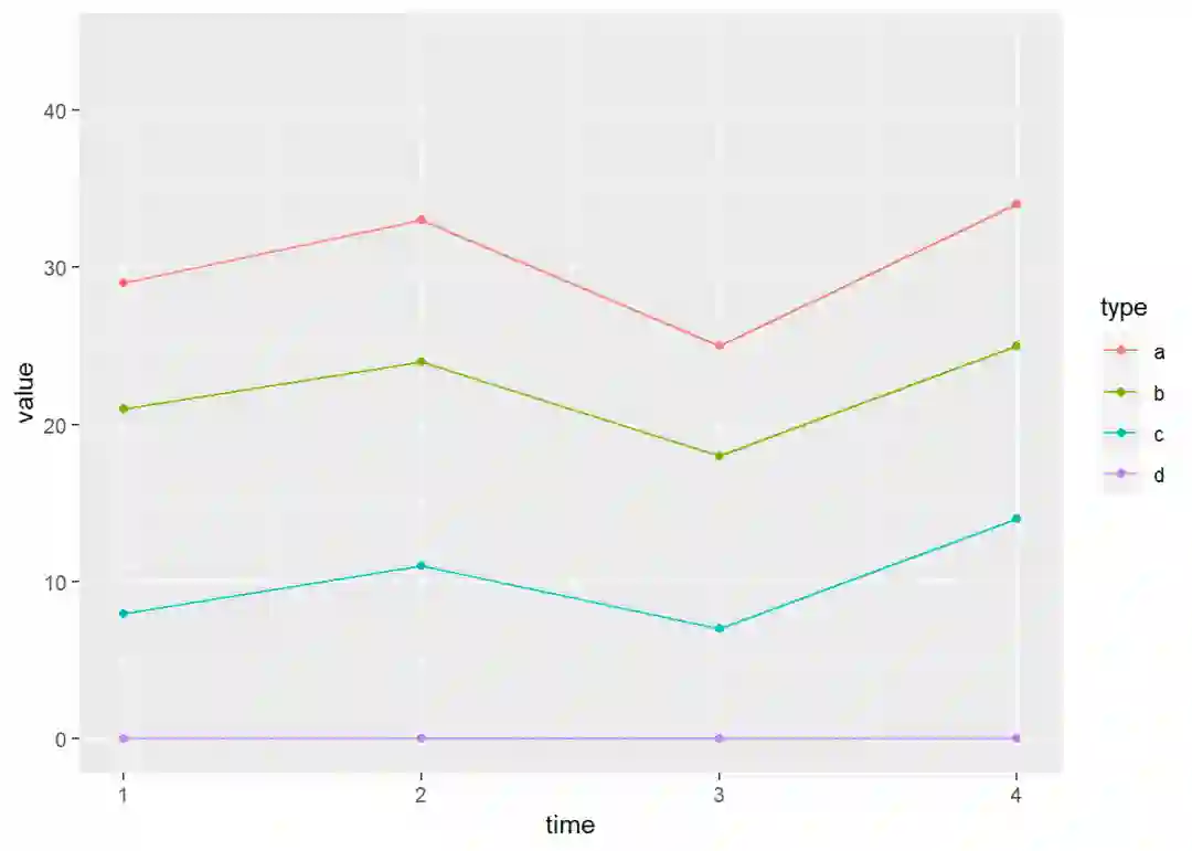
ggplot(series, aes(time, value, group = type)) + geom_line(aes(colour = type),
position = position_stack(vjust = 0.5)) + geom_point(aes(colour = type),
position = position_stack(vjust = 0.5)) # 向下移动半个单位,以最下面的元素为高度为基准
ggplot(series, aes(time, value, group = type)) + geom_line(aes(colour = type),
position = position_stack(vjust = 0)) + geom_point(aes(colour = type), position = position_stack(vjust = 0)) # 向下移动到底,最下面的折线都拉直了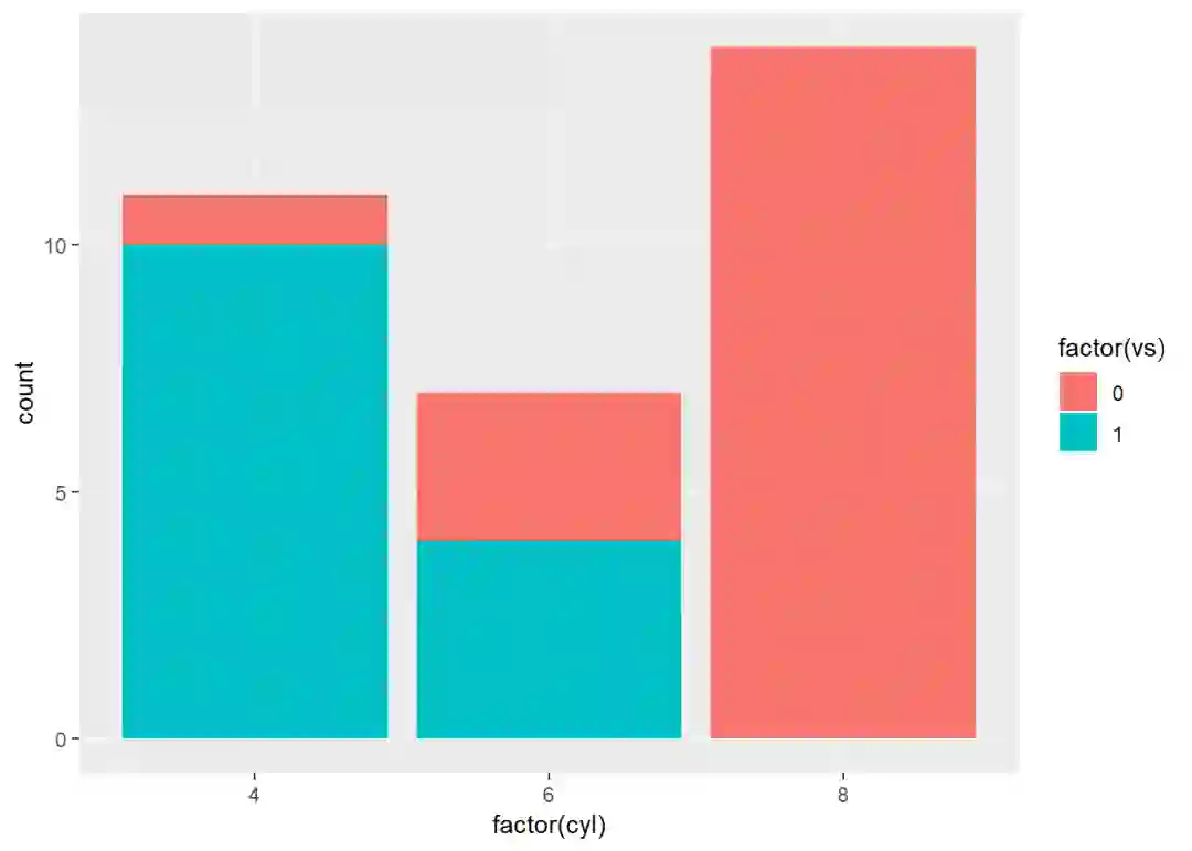
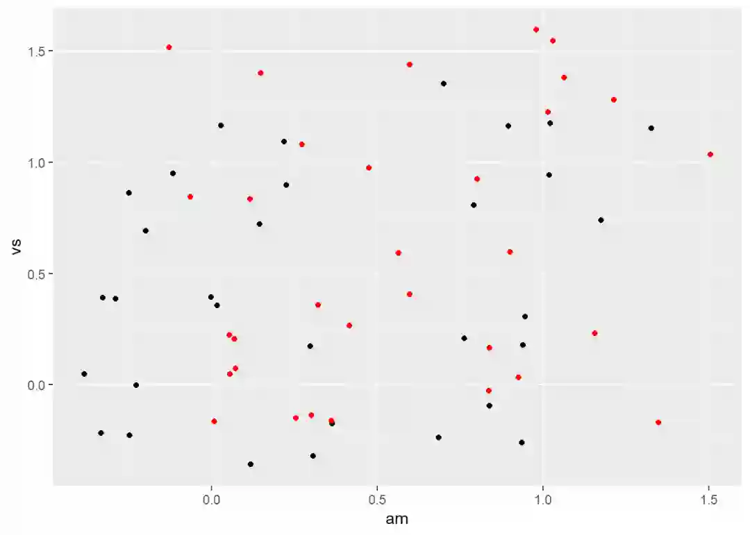
4.2.3 position_jitter(), position_jitterdodge() 扰动错开
library(ggplot2)
ggplot(mtcars, aes(am, vs)) +
geom_jitter()
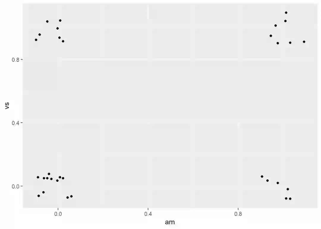
ggplot(mtcars, aes(am, vs)) +
geom_jitter(width = 0.1, height = 0.1) # 增加水平抖动10%,垂直抖动10%
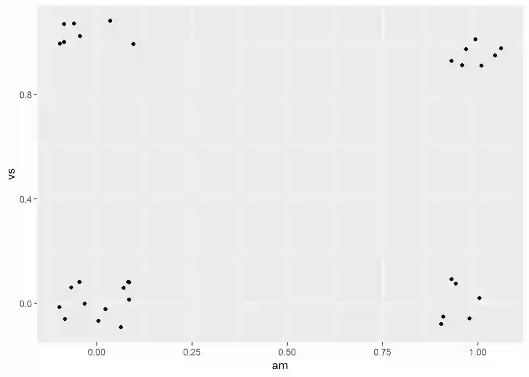
ggplot(mtcars, aes(am, vs)) +
geom_point(position = position_jitter(width = 0.1, height = 0.1)) # 原理与上面一样,但是抖动是随机的,每次结果都可能不一样
ggplot(mtcars, aes(am, vs)) +
geom_point(position = "jitter") + # 默认抖动50%
geom_point(aes(am + 0.2, vs + 0.2), position = "jitter", color = "red" ) # 可以在映射里面进行简单的运算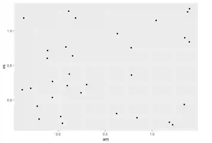
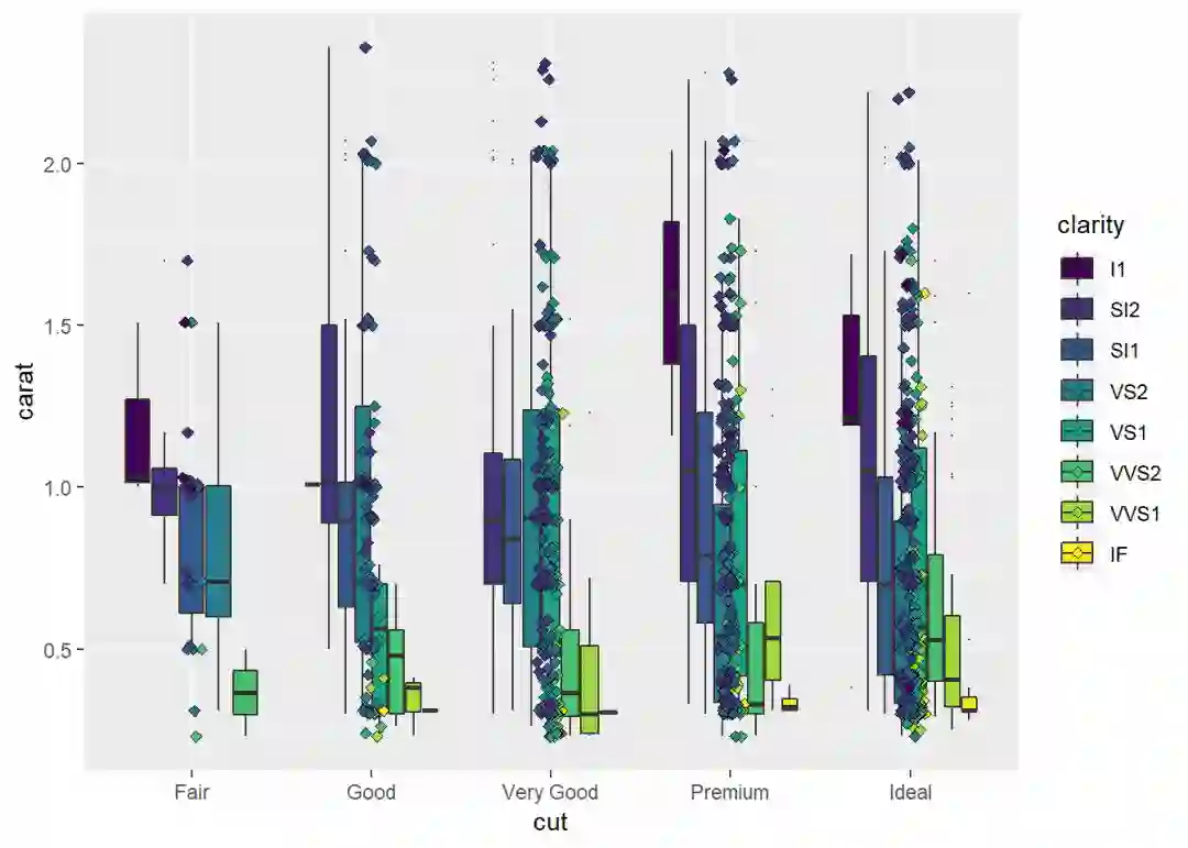
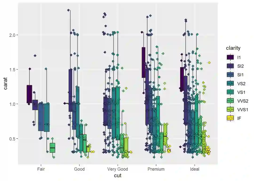
4.2.4 position_jitterdodge()
position_jitterdodge(jitter.width = NULL, jitter.height = 0, dodge.width = 0.75, seed = NA)
仅仅用于箱线图和点图在一起的情形,且有顺序的,必须箱子在前,点图在后,抖动只能用在散点几何对象中,
jitter.width 默认40%, jitter.height 默认0
library(ggplot2)
dsub <- diamonds[sample(nrow(diamonds), 1000), ]

ggplot(dsub, aes(x = cut, y = carat, fill = clarity)) + geom_boxplot(outlier.size = 0) +
    geom_point(shape = 23)  # 23号点形状为菱形

ggplot(dsub, aes(x = cut, y = carat, fill = clarity)) + geom_boxplot(outlier.size = 0) +
    geom_point(shape = 23, position = position_jitterdodge(dodge.width = 0.1))  # 点分布于各组箱子10%宽度上,默认点水平抖动错开

ggplot(dsub, aes(x = cut, y = carat, fill = clarity)) + geom_boxplot(outlier.size = 0) +
    geom_point(shape = 23, position = position_jitterdodge(dodge.width = 0.8))  # 点分布于各组箱子80%宽度上,默认点水平抖动错开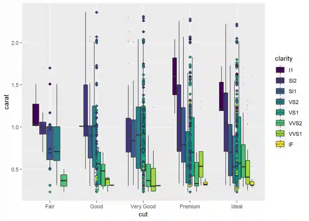
4.2.5 position_nudge 整体微调
library(ggplot2)
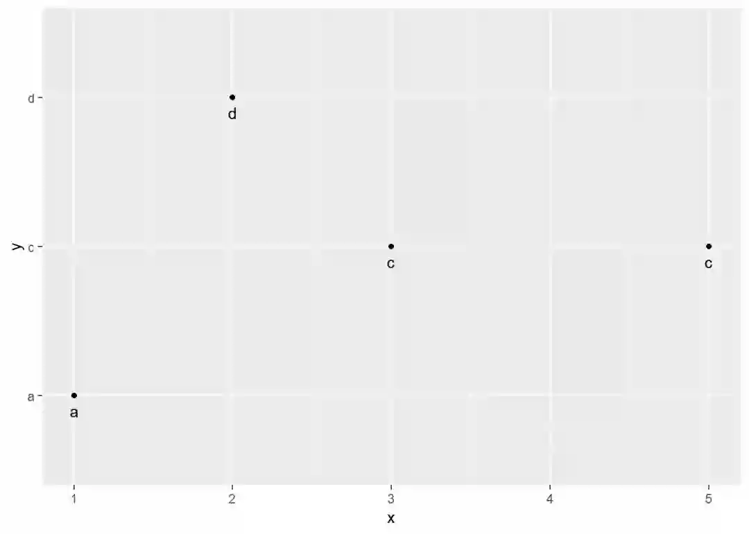
df <- data.frame(x = c(1, 3, 2, 5), y = c("a", "c", "d", "c"))
ggplot(df, aes(x, y)) + geom_point() + geom_text(aes(label = y)) # 文本对象位置与点重合,视觉效果不好
ggplot(df, aes(x, y)) + geom_point() + geom_text(aes(label = y), position = position_nudge(y = -0.1)) # 文本位置向下移动1%个单位,错开文本与点位置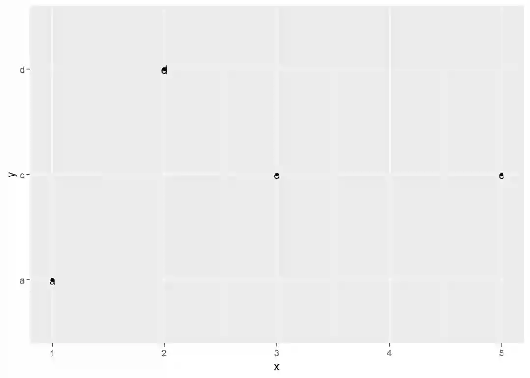


公众号后台回复关键字即可学习
回复 爬虫 爬虫三大案例实战
回复 Python 1小时破冰入门回复 数据挖掘 R语言入门及数据挖掘
回复 人工智能 三个月入门人工智能
回复 数据分析师 数据分析师成长之路
回复 机器学习 机器学习的商业应用
回复 数据科学 数据科学实战
回复 常用算法 常用数据挖掘算法