一文教你如何用PyTorch构建 Faster RCNN

本文为 AI 研习社编译的技术博客，原标题 ：

Guide to build Faster RCNN in PyTorch

作者 | Machine-Vision Research Group

翻译 | 邓普斯•杰弗、麦尔肯•诺埃、莫青悠

校对 | 邓普斯•杰弗       审核 | 酱番梨      整理 | 菠萝妹

原文链接：

https://medium.com/@fractaldle/guide-to-build-faster-rcnn-in-pytorch-95b10c273439

注：本文共31000+字，建议收藏阅读。相关链接请点击文末【阅读原文】进行访问。

一文教你如何用PyTorch构建 Faster RCNN

  引言

Faster R-CNN是首次完全采用Deep Learning的学习框架之一。Faster R-CNN是基于Fast RCNN的思路，然而Fast RCNN却继承自RCNN，SPP-Net的思路（译者注：此处理清楚先后关系）。虽然我们在构建Faster RCNN框架时引入了一些Fast RCNN的思想，但是我们不会详细讨论这些框架。其中一个原因是，Faster R-CNN表现得非常好，它没有使用传统的计算机视觉技术，如选择性搜索等。在非常高的层次上，Fast RCNN和Faster RCNN的工作原理如下面的流程图所示。

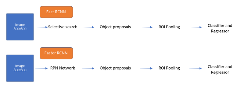
Fast RCNN和Faster RCNN  

我们写过一篇关于目标检测框架的详细的博客，可以作为独自编码理解Faster RCNN的指导。

上图可以看到唯一的区别是Faster RCNN中将selective search替换为RPN(Region Proposal Network)，selective search算法采用SIFT和HOG描述子来生成目标候选，在CPU上2秒/张图像。这一过程代价高，Fast RCNN在一张图像上总共耗费2.3秒产生预测，Faster RCNN速度为5 FPS（每秒的帧数），即使在后端使用非常深入的图像分类器，如VGGnet(现在也使用ResNet和ResNext)。

 因此，为了从零开始构建Faster RCNN，需要明确理解以下4个主题（流程）：

1. Region Proposal network (RPN)

2. RPN loss functions

3. Region of Interest Pooling (ROI)

4. ROI loss functions

RPN还引入了一个新的概念：Anchor boxes，这成为构建目标检测框架的一个黄金准则。下面我们深入理解目标检测框架的不同步骤在Faster RCNN中如何发挥作用。

在训练Faster RCNN时通常的数据流如下：

1.  从图像中提取特征；

2.  产生anchor目标；

3.  RPN网络中得到位置和目标预测分值；

4. 取前N个坐标及其目标得分即建议层；

5.  传递前N个坐标通过Fast R-CNN网络，生成4中建议的每个位置的位置和cls预测；

6.  对4中建议的每个坐标生成建议目标；

7.  采用2,3计算rpn_cls_loss和rpn_reg_loss；

8.  采用5,6计算roi_cls_loss和roi_reg_loss；

配置VGG16作为实验后期的网络，可以用相似的方式采用其他任意的分类网络。

  特征提取

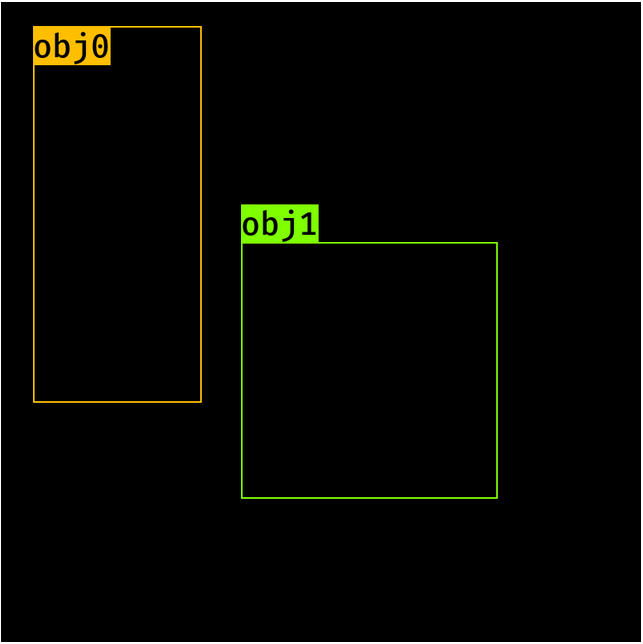
我们从一张图像和一组边界框开始，其标签定义如下：

import torch
image = torch.zeros((1, 3, 800, 800)).float()

bbox = torch.FloatTensor([[20, 30, 400, 500], [300, 400, 500, 600]]) 

# [y1, x1, y2, x2] format
labels = torch.LongTensor([6, 8]) # 0 represents background
sub_sample = 16

VGG16网络作为特征提取模块，这是RPN和Fast RCNN的支柱，为此需要对VGG16网络进行修改，网络输入为800，特征提取模块的输出的特征图尺寸为（800//16），因此需要保证VGG16模块可以得到这样的特征图储存并且将网络修剪整齐，可以通过如下方式实现：

• 创建一个dummy image，并将volatile设置为False;

• 列出VGG16所有的层；

• 当图像(feature map)的output_size低于所需的级别(800//16)时，将图像传递到各个层并对列表取子集；

• 将list转换为Sequential module;

来看看每个步骤：

1. 生成一个dummy image并且设置volatile为False：

import torchvision
dummy_img = torch.zeros((1, 3, 800, 800)).float()
print(dummy_img)
#Out: torch.Size([1, 3, 800, 800])

2. 列出VGG16的所有层：

model = torchvision.models.vgg16(pretrained=True)
fe = list(model.features)

print(fe) # length is 15
# [Conv2d(3, 64, kernel_size=(3, 3), stride=(1, 1), padding=(1, 1)),
#  ReLU(inplace),
#  Conv2d(64, 64, kernel_size=(3, 3), stride=(1, 1), padding=(1, 1)),
#  ReLU(inplace),
#  MaxPool2d(kernel_size=(2, 2), stride=(2, 2), dilation=(1, 1), ceil_mode=False),
#  Conv2d(64, 128, kernel_size=(3, 3), stride=(1, 1), padding=(1, 1)),
#  ReLU(inplace),
#  Conv2d(128, 128, kernel_size=(3, 3), stride=(1, 1), padding=(1, 1)),
#  ReLU(inplace),
#  MaxPool2d(kernel_size=(2, 2), stride=(2, 2), dilation=(1, 1), ceil_mode=False),
#  Conv2d(128, 256, kernel_size=(3, 3), stride=(1, 1), padding=(1, 1)),
#  ReLU(inplace),
#  Conv2d(256, 256, kernel_size=(3, 3), stride=(1, 1), padding=(1, 1)),
#  ReLU(inplace),
#  Conv2d(256, 256, kernel_size=(3, 3), stride=(1, 1), padding=(1, 1)),
#  ReLU(inplace),
#  MaxPool2d(kernel_size=(2, 2), stride=(2, 2), dilation=(1, 1), ceil_mode=False),
#  Conv2d(256, 512, kernel_size=(3, 3), stride=(1, 1), padding=(1, 1)),
#  ReLU(inplace),
#  Conv2d(512, 512, kernel_size=(3, 3), stride=(1, 1), padding=(1, 1)),
#  ReLU(inplace),
#  Conv2d(512, 512, kernel_size=(3, 3), stride=(1, 1), padding=(1, 1)),
#  ReLU(inplace),
#  MaxPool2d(kernel_size=(2, 2), stride=(2, 2), dilation=(1, 1), ceil_mode=False),
#  Conv2d(512, 512, kernel_size=(3, 3), stride=(1, 1), padding=(1, 1)),
#  ReLU(inplace),
#  Conv2d(512, 512, kernel_size=(3, 3), stride=(1, 1), padding=(1, 1)),
#  ReLU(inplace),
#  Conv2d(512, 512, kernel_size=(3, 3), stride=(1, 1), padding=(1, 1)),
#  ReLU(inplace),
#  MaxPool2d(kernel_size=(2, 2), stride=(2, 2), dilation=(1, 1), ceil_mode=False)]

3. 将图像传输通过所有层，确定得到相应的尺寸：

req_features = []
k = dummy_img.clone()
for i in fe:
    k = i(k)
    if k.size()[2] < 800//16:
        break
    fee.append(i)
    out_channels = k.size()[1]
print(len(req_features)) #30
print(out_channels) # 512

4. 将list转换为Sequential module：

faster_rcnn_fe_extractor = nn.Sequential(*req_features)

现在faster_rcnn_fe_extractor可以作为后端，计算特征：

out_map = faster_rcnn_fe_extractor(image)
print(out_map.size())
#Out: torch.Size([1, 512, 50, 50])

  Anchor boxes

这是我们第一次遇到anchor boxes。详细理解将使我们能够非常容易地理解目标检测。所以让我们详细谈谈这是如何做到的。  

1.  在一个feature map的坐标上生成Anchor；

2. 在所有feature map的坐标上生成Anchor；

3. 对每个目标分配标签及坐标（相对于anchor）；

4.  在feature map坐标生成Anchor；

• 将采用anchor_scales=8，16，32，ratio=0.5，1，2，sub sampling=16（因为我们将图像从800像素池化至50像素）。输出的feature map的每个像素对应图像中的16*16像素，如下图所示：

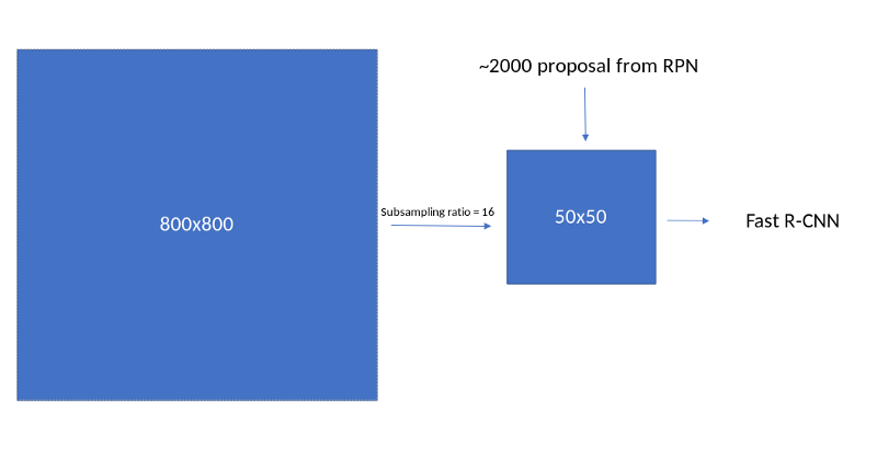
image to feature map mapping

• 我们需要首先在这个16 * 16像素上生成锚框，然后沿着x轴和y轴进行类似的操作，以获得所有的anchor boxes。这在步骤2中完成。  

• feature map的每个像素位置生成9个anchor boxes（anchor_scales的数量和ratio的数量），每个anchor box具有‘y1’,‘x1’,‘y2’,‘x2’。因此每个位置anchor会具有形状（9,4）。开始为一个空的全0的数组。

import numpy as np
ratio = [0.5, 1, 2]
anchor_scales = [8, 16, 32]

anchor_base = np.zeros((len(ratios) * len(scales), 4), dtype=np.float32)

print(anchor_base)

#Out:
# array([[0., 0., 0., 0.],
#        [0., 0., 0., 0.],
#        [0., 0., 0., 0.],
#        [0., 0., 0., 0.],
#        [0., 0., 0., 0.],
#        [0., 0., 0., 0.],
#        [0., 0., 0., 0.],
#        [0., 0., 0., 0.],
#        [0., 0., 0., 0.]], dtype=float32)

让我们用相应的y1、x1、y2、x2填充这些值。我们的这个基础anchor的中心将在：  

ctr_y = sub_sample / 2.
ctr_x = sub_sample / 2.

print(ctr_y, ctr_x)
# Out: (8, 8)
for i in range(len(ratios)):
  for j in range(len(anchor_scales)):
    h = sub_sample * anchor_scales[j] * np.sqrt(ratios[i])
    w = sub_sample * anchor_scales[j] * np.sqrt(1./ ratios[i])

    index = i * len(anchor_scales) + j

    anchor_base[index, 0] = ctr_y - h / 2.
    anchor_base[index, 1] = ctr_x - w / 2.
    anchor_base[index, 2] = ctr_y + h / 2.
    anchor_base[index, 3] = ctr_x + w / 2.

#Out:
# array([[ -37.254833,  -82.50967 ,   53.254833,   98.50967 ],
#        [ -82.50967 , -173.01933 ,   98.50967 ,  189.01933 ],
#        [-173.01933 , -354.03867 ,  189.01933 ,  370.03867 ],
#        [ -56.      ,  -56.      ,   72.      ,   72.      ],
#        [-120.      , -120.      ,  136.      ,  136.      ],
#        [-248.      , -248.      ,  264.      ,  264.      ],
#        [ -82.50967 ,  -37.254833,   98.50967 ,   53.254833],
#        [-173.01933 ,  -82.50967 ,  189.01933 ,   98.50967 ],
#        [-354.03867 , -173.01933 ,  370.03867 ,  189.01933 ]],
#       dtype=float32)

这些是第一个feature map像素的Anchor位置，我们现在必须在feature map的所有位置生成这些anchor。还要注意，negitive值表示anchor boxes在图像维度之外。在后面的部分中，我们将用-1标记它们，并在计算函数损失和生成Anchor建议时删除它们。而且由于我们在每个位置都有9个Anchor，并且在一个图像中有50 * 50个这样的位置，我们总共会得到17500个(50 * 50 * 9) Anchor。让我们现在生成其他Anchor 。（译者注：此处生成的是备选Anchor，即所有可能的Anchor）

2. 在所有特征图位置生成Anchor

为了实现这一目标，首先需要为每个feature map像素生成中心（复原到原始图像的位置点）：

fe_size = (800//16)
ctr_x = np.arange(16, (fe_size+1) * 16, 16)
ctr_y = np.arange(16, (fe_size+1) * 16, 16)

遍历ctr_x和ctr_y可以得到每个位置的中心，代码如下：

For x in shift_x:
 For y in shift_y:
   Generate anchors at (x, y) locations

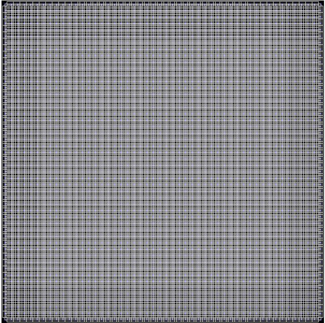
anchor中心可视化如下：

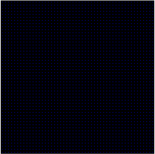
图像中的anchor中心

采用python生成中心：

index = 0
for x in range(len(ctr_x)):
    for y in range(len(ctr_y)):
        ctr[index, 1] = ctr_x[x] - 8
        ctr[index, 0] = ctr_y[y] - 8
        index +=1

• 输出将是每个位置的(x, y)值，如上图所示。我们总共有2500个锚点。现在我们需要在每个中心生成anchor boxes。这可以使用我们在一个位置生成锚的代码来完成，为提供每个anchor中心的代码添加一个提取for循环就可以了。让我们看看这是怎么做的：

anchors = np.zeros((fe_size * fe_size * 9), 4)

index = 0
for c in ctr:
  ctr_y, ctr_x = c
  for i in range(len(ratios)):
    for j in range(len(anchor_scales)):
      h = sub_sample * anchor_scales[j] * np.sqrt(ratios[i])
      w = sub_sample * anchor_scales[j] * np.sqrt(1./ ratios[i])
      anchors[index, 0] = ctr_y - h / 2.
      anchors[index, 1] = ctr_x - w / 2.
      anchors[index, 2] = ctr_y + h / 2.
      anchors[index, 3] = ctr_x + w / 2.
      index += 1
print(anchors.shape)
#Out: [22500, 4]

注：为了简单起见，我让这段代码看起来非常冗长。有更好的方法来生成anchor boxes。

这会成为图像最终的anchor用于后续的步骤，下面可视化这些anchor如何 在图像上传播。

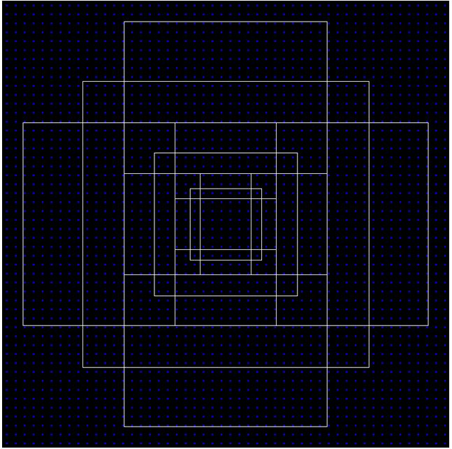
anchor boxes at (400, 400)：

一张图像中所有有效的anchor boxes示意图

1. 分配目标标签和位置给每个anchor

现在，由于我们已经生成了所有的anchor boxes，我们需要查看图像中的目标，并将它们分配给包含它们的特定anchor boxes。Faster_R-CNN有一些给anchor boxes分配标签的指导原则。

我们给两种anchor分配了正标签：

 a)与ground-truth-box重叠度最高的Intersection-over-Union (IoU)的anchor；

b)与ground-truth box   的IoU重叠度大于0.7的anchor。

注意，单个ground-truth对象可以为多个anchor分配正标签。

c)对所有与ground-truth box的IoU比率小于0.3的anchor标记为负标签；  

d)anchor既不是正样本的也不是负样本，对训练没有帮助。

让我们看看这是怎么做的。 

bbox = np.asarray([[20, 30, 400, 500], [300, 400, 500, 600]], 
dtype=np.float32) # [y1, x1, y2, x2] format
labels = np.asarray([6, 8], dtype=np.int8) # 0 represents background

通过如下方式对anchor boxes分配标签和位置：

• 找到有效的anchor boxes的索引，并且生成索引数组，生成标签数组其形状索引数组填充-1（无效anchor boxes，对应上文说的处在边框外的anchor boxes）。

• 检查是否满足以上a、b、c条件中的一条，并相应填写标签。如果是正anchor box(标签为1)，注意哪个ground-truth目标可以得到这个结果。

• 计算与anchor box相关的ground-truth的位置(loc)。

• 通过为所有无效的anchor box填充-1和为所有有效锚箱计算的值来重新组织所有锚箱。

• 输出应该是(N, 1)数组的标签和带有(N, 4)数组的locs。

• 找到所有有效anchor boxes的索引：

index_inside = np.where(
        (anchors[:, 0] >= 0) &
        (anchors[:, 1] >= 0) &
        (anchors[:, 2] <= 800) &
        (anchors[:, 3] <= 800)
    )[0]
print(index_inside.shape)
#Out: (8940,)

• 生成空的标签数组，大小为inside_index，填充-1，默认设置为(d)：

label = np.empty((len(inside_index), ), dtype=np.int32)
 label.fill(-1)
 print(label.shape)
#Out = (8940, )

• 生成有效anchor boxes数组：

valid_anchor_boxes = anchors[inside_index]
print(valid_anchor_boxes.shape)
#Out = (8940, 4)

• 对每个有效anchor box计算与每个ground-truth目标的iou。因为我们有8940个anchor boxes和2个ground-truth目标，应该得到（8940,2）的数组作为输出。两个框之间iou计算的代码如下：

- Find the max of x1 and y1 in both the boxes (xn1, yn1)
- Find the min of x2 and y2 in both the boxes (xn2, yn2)
- Now both the boxes are intersecting only
if (xn1 < xn2) and (yn2 < yn1)
     - iou_area will be (xn2 - xn1) * (yn2 - yn1)
else 
     - iuo_area will be 0
 - similarly calculate area for anchor box and ground truth object
- iou = iou_area/(anchor_box_area + ground_truth_area - iou_area)

计算iou的python代码如下：

ious = np.empty((len(valid_anchors), 2), dtype=np.float32)
ious.fill(0)
print(bbox)
for num1, i in enumerate(valid_anchors):
    ya1, xa1, ya2, xa2 = i 
    anchor_area = (ya2 - ya1) * (xa2 - xa1)
    for num2, j in enumerate(bbox):
        yb1, xb1, yb2, xb2 = j
        box_area = (yb2- yb1) * (xb2 - xb1)

        inter_x1 = max([xb1, xa1])
        inter_y1 = max([yb1, ya1])
        inter_x2 = min([xb2, xa2])
        inter_y2 = min([yb2, ya2])
        if (inter_x1 < inter_x2) and (inter_y1 < inter_y2):
            iter_area = (inter_y2 - inter_y1) * \
(inter_x2 - inter_x1)
            iou = iter_area / \
(anchor_area+ box_area - iter_area) 
        else:
            iou = 0.

        ious[num1, num2] = iou
print(ious.shape)
#Out: [22500, 2]

注意：采用numpy数组，可以使计算效率更高并且冗余更少。然而，我们这样做的原因是可以使没有很强的代数知识的人也能理解。

考虑a和b的情况，我们需要找到两件事

1. 每个gt_box及其对应的anchor box的最高iou；

2. 每个anchor box及其对应的ground-truth box的最高iou；  

case-1：

gt_argmax_ious = ious.argmax(axis=0)
print(gt_argmax_ious)
gt_max_ious = ious[gt_argmax_ious, np.arange(ious.shape[1])]
print(gt_max_ious)
# Out:
# [2262 5620]
# [0.68130493 0.61035156]

case-2：

argmax_ious = ious.argmax(axis=1)
print(argmax_ious.shape)
print(argmax_ious)
max_ious = ious[np.arange(len(inside_index)), argmax_ious]
print(max_ious)
# Out:
# (22500,)
# [0, 1, 0, ..., 1, 0, 0]
# [0.06811669 0.07083762 0.07083762 ... 0.         0.         0.        ]

找到具有max_ious的anchor_boxes（gt_max_ious）：

gt_argmax_ious = np.where(ious == gt_max_ious)[0]
print(gt_argmax_ious)
# Out:
# [2262, 2508, 5620, 5628, 5636, 5644, 5866, 5874, 5882, 5890, 6112,
#        6120, 6128, 6136, 6358, 6366, 6374, 6382]

至此有3个数组：

• argmax_ious——确定哪个ground-truth目标与每个anchor都有最大的iou；

• max_ious——确定ground-truth目标与每个anchor的max_iou；

• gt_argmax_ious——确定与ground-truth box有最大的IoU重叠的anchor。

用argmax_ious和max_ious可以为满足[b],[c]的anchor box分配标签和位置，使用gt_argmax_iou，我们可以为anchor box分配标签和位置，以满足[a]。

 对一些变量施加阈值：

pos_iou_threshold  = 0.7
neg_iou_threshold = 0.3

• 分配负标签（0）给max_iou小于负阈值[c]的所有anchor boxes：

label[max_ious < neg_iou_threshold] = 0

• 分配正标签（1）给与ground-truth box[a]的IoU重叠最大的anchor boxes：

label[gt_argmax_ious] = 1

• 分配正标签（1）给max_iou大于positive阈值[b]的anchor boxes：

label[max_ious >= pos_iou_threshold] = 1

训练RPN，Faster_R-CNN文章描述如下：

每个mini-batch都来自包含许多正样本和负样本anchor的单个图像，但这将偏向负样本，因为它们占主导地位。相反，我们随机采样图像中的256个anchor来计算mini-batch的损失函数，其中被采样的正锚点和负锚点的比例高达1:1。如果一幅图像中有少于128个正样本，我们就用负样本填充mini-batch图像。由此我们可以推出两个变量如下 ：

pos_ratio = 0.5
n_sample = 256

所有的正样本 ：

n_pos = pos_ratio * n_sample

现在我们需要从正标签中随机采样n_pos个样本，忽略（-1）剩余的样本。在一些情况下，得到少于n_pos个样本，此时随机采样（n_sample-n_pos）个负样本（0），忽略剩余的anchor boxes，用如下代码实现：

• positive samples

pos_index = np.where(label == 1)[0]
if len(pos_index) > n_pos:
    disable_index = np.random.choice(pos_index, size=(len(pos_index) - n_pos), replace=False)
    label[disable_index] = -1

• negative samples

n_neg = n_sample * np.sum(label == 1)
neg_index = np.where(label == 0)[0]
if len(neg_index) > n_neg:
    disable_index = np.random.choice(neg_index, size=(len(neg_index) - n_neg), replace = False)
    label[disable_index] = -1

  anchor boxes 定位

现在让我们用具有最大iou的ground truth对象为每个anchor box分配位置。注意，我们将为所有有效的anchor box分配anchor locs，而不考虑其标签，稍后在计算损失时，我们可以使用简单的过滤器删除它们。

我们已经知道与每个anchor box具有高的iou的ground truth目标，现在我们需要找到ground truth相对于anchor box的坐标。Faster_R-CNN按照如下参数化：

t_{x} = (x - x_{a})/w_{a}
t_{y} = (y - y_{a})/h_{a}
t_{w} = log(w/ w_a)
t_{h} = log(h/ h_a)

x, y , w, h是ground truth box的中心坐标，宽，高。x_a，y_a，h_a，w_a为anchor boxes的中心坐标，宽，高。

• 对每个anchor box，找到具有max_iou的ground-truth目标：

max_iou_bbox = bbox[argmax_ious]
print(max_iou_bbox)
#Out
# [[ 20.,  30., 400., 500.],
#  [ 20.,  30., 400., 500.],
#  [ 20.,  30., 400., 500.],
#  ...,
#  [ 20.,  30., 400., 500.],
#  [ 20.,  30., 400., 500.],
#  [ 20.,  30., 400., 500.]]

• 为找到t_{x}, t_{y}, t_{w}, t_{h}，需要转换有效的anchor boxes的y1,x1,y2,x2格式和与ground truth boxes相关的ctr_y，ctr_x，h，w格式：

height = valid_anchors[:, 2] - valid_anchors[:, 0]
width = valid_anchors[:, 3] - valid_anchors[:, 1]
ctr_y = valid_anchors[:, 0] + 0.5 * height
ctr_x = valid_anchors[:, 1] + 0.5 * width
base_height = max_iou_bbox[:, 2] - max_iou_bbox[:, 0]
base_width = max_iou_bbox[:, 3] - max_iou_bbox[:, 1]
base_ctr_y = max_iou_bbox[:, 0] + 0.5 * base_height
base_ctr_x = max_iou_bbox[:, 1] + 0.5 * base_width

• 用上述公式找到位置：

eps = np.finfo(height.dtype).eps
height = np.maximum(height, eps)
width = np.maximum(width, eps)
dy = (base_ctr_y - ctr_y) / height
dx = (base_ctr_x - ctr_x) / width
dh = np.log(base_height / height)
dw = np.log(base_width / width)
anchor_locs = np.vstack((dy, dx, dh, dw)).transpose()
print(anchor_locs)
#Out:
# [[ 0.5855727   2.3091455   0.7415673   1.647276  ]
#  [ 0.49718437  2.3091455   0.7415673   1.647276  ]
#  [ 0.40879607  2.3091455   0.7415673   1.647276  ]
#  ...
#  [-2.50802    -5.292254    0.7415677   1.6472763 ]
#  [-2.5964084  -5.292254    0.7415677   1.6472763 ]
#  [-2.6847968  -5.292254    0.7415677   1.6472763 ]]

• 现在得到anchor_locs和与每个有效的anchor boxes相关的标签

用inside_index变量将他们映射到原始的anchors，无效的anchor box标签填充-1（忽略），位置填充0。

• 最终的标签：

anchor_labels = np.empty((len(anchors),), dtype=label.dtype)
anchor_labels.fill(-1)
anchor_labels[inside_index] = label

最终的坐标：

anchor_locations = np.empty((len(anchors),) + anchors.shape[1:], dtype=anchor_locs.dtype)
anchor_locations.fill(0)
anchor_locations[inside_index, :] = anchor_locs

最终的两个矩阵为：

• anchor_locations [N, 4] — [22500, 4]

• anchor_labels [N,] — [22500]

这用于RPN网络的输入目标，下节可以看到RPN网络如何设计。

  Region Proposal Network（RPN网络）

正如之前讨论，在先前的研究中，通过selective search，CPMC, MCG, EdgeBoxes等方法生成网络的region proposals。Faster R-CNN是第一个采用深度学习生成region proposals的方法。

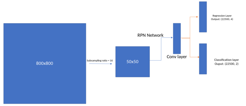
RPN Network

网络包括一个卷积模块，在卷积模块下一层包括一个回归层，预测anchor中的box的位置。

为生成region proposals，在特征提取模块得到的卷积特征层输出上滑动一个小的网络。这个小网络将输入卷积特征层的n*n空间窗口作为输入，每个滑动窗口映射到更低维的特征[512维特征]。这个特征输入到两个并列的全连接层：

• 框回归层
  

• 框分类层
  

正如Faster R-CNN文章中所属，采用n=3，采用n*n的卷积层和两个并列的1*1卷积层实现这一框架：

import torch.nn as nn
mid_channels = 512
in_channels = 512 # depends on the output feature map. in vgg 16 it is equal to 512
n_anchor = 9 # Number of anchors at each location
conv1 = nn.Conv2d(in_channels, mid_channels, 3, 1, 1)
reg_layer = nn.Conv2d(mid_channels, n_anchor *4, 1, 1, 0)
cls_layer = nn.Conv2d(mid_channels, n_anchor *2, 1, 1, 0) ## I will 
be going to use softmax here. you can equally use sigmoid if u 
replace 2 with 1.

文章中，采用均值0，标准差0.01初始化权重，偏差初始化为0，通过如下代码实现：

# conv sliding layer
conv1.weight.data.normal_(0, 0.01)
conv1.bias.data.zero_()

# Regression layer
reg_layer.weight.data.normal_(0, 0.01)
reg_layer.bias.data.zero_()

# classification layer
cls_layer.weight.data.normal_(0, 0.01)
cls_layer.bias.data.zero_()

特征提取过程的输出可以输入到网络中用于预测目标相对anchor的位置和与之相关的目标分值：

x = conv1(out_map) # out_map is obtained in section 1
pred_anchor_locs = reg_layer(x)
pred_cls_scores = cls_layer(x)

print(pred_cls_scores.shape, pred_anchor_locs.shape)

#Out:
#torch.Size([1, 18, 50, 50]) torch.Size([1, 36, 50, 50])

让我们重新格式化一下，让它与我们之前设计的锚点目标对齐。我们还将找到每个anchor box的目标得分用于proposal层，我们将在下一节中讨论：

pred_anchor_locs = pred_anchor_locs.permute(0, 2, 3, 1).contiguous().view(1, -1, 4)
print(pred_anchor_locs.shape)

#Out: torch.Size([1, 22500, 4])

pred_cls_scores = pred_cls_scores.permute(0, 2, 3, 1).contiguous()
print(pred_cls_scores)
#Out torch.Size([1, 50, 50, 18])

objectness_score = pred_cls_scores.view(1, 50, 50, 9, 2)[:, :, :, :, 1].contiguous().view(1, -1)
print(objectness_score.shape)
#Out torch.Size([1, 22500])

pred_cls_scores  = pred_cls_scores.view(1, -1, 2)
print(pred_cls_scores.shape)
# Out torch.size([1, 22500, 2])

本节实现以下步骤：

• pred_cls_scores和pred_anchor_locs是RPN网络的输出，损失更新权重。

• pred_cls_scores和objectness_scores作为proposal层的输入，proposal层生成后续用于RoI网络的一系列proposal，将在下一节中实现。

  Generating proposals to feed Fast R-CNN network

proposal函数将采用如下参数：

• 模式：training_mode还是testing_mode。

• nms_thresh。

• n_train_pre_nms——训练时nms之前的bbox的数目。

• n_train_post_nms——训练时nms之后的bbox的数目。

• n_test_pre_nms——测试时nms之前的bbox的数目。

• n_test_post_nms——测试时nms之后的bbox的数目。

• min_size——生成一个proposal的所需的目标的最小高度。

Faster R-CNN中RPN的proposals彼此之间重叠程度高。为了减少冗余，我们根据proposal区域的cls分数对其进行非最大抑制(non-maximum supression, NMS)。我们将NMS的IoU阈值设置为0.7，这样每个图像就有大约2000个建议区域。经过简化研究，作者表明，NMS不损害最终检测的准确性，但大大减少了建议的数量。在NMS之后，我们使用top-N的建议区域进行检测。后续使用2000个RPN proposals训练Fast R-CNN。在测试期间，他们只评估了300个proposal，他们用不同的数字测试，并得到了如下结果：

nms_thresh = 0.7
n_train_pre_nms = 12000
n_train_post_nms = 2000
n_test_pre_nms = 6000
n_test_post_nms = 300
min_size = 16

我们需要做以下的事情产生网络感兴趣的proposal region。

1. 转换RPN网络的loc预测为bbox[y1,x1,y2,x2]格式。

2. 将预测框剪辑到图像上。

3. 去除高度或宽度

4. 通过分数从高到低排序所有的(proposal, score)对。

5. 取前几个预测框pre_nms_topN(如，训练时12000，测试时300)

6. 采用nms threshold > 0.7。

7. 取前几个预测框pos_nms_topN(如，训练时2000，测试时300)

我们将在本节剩余部分中查看每个阶段：

1. 转换RPN网络的loc预测为bbox[y1,x1,y2,x2]格式。  

这是为anchor boxes设置ground truth时的逆操作，该操作通过无参数化及相对图像的偏差来解码预测。公式如下：

x = (w_{a} * ctr_x_{p}) + ctr_x_{a}
y = (h_{a} * ctr_x_{p}) + ctr_x_{a}
h = np.exp(h_{p}) * h_{a}
w = np.exp(w_{p}) * w_{a}

and later convert to y1, x1, y2, x2 format

• 转换anchor格式从 y1, x1, y2, x2 到 ctr_x, ctr_y, h, w  ：

anc_height = anchors[:, 2] - anchors[:, 0]
anc_width = anchors[:, 3] - anchors[:, 1]
anc_ctr_y = anchors[:, 0] + 0.5 * anc_height
anc_ctr_x = anchors[:, 1] + 0.5 * anc_width

• 通过上述公式转换预测locs，在转换之前先将pred_anchor_loc和objectness_score为numpy数组：

pred_anchor_locs_numpy = pred_anchor_locs[0].data.numpy()
objectness_score_numpy = objectness_score[0].data.numpy()

dy = pred_anchor_locs_numpy[:, 0::4]
dx = pred_anchor_locs_numpy[:, 1::4]
dh = pred_anchor_locs_numpy[: 2::4]
dw = pred_anchor_locs_numpy[: 3::4]

ctr_y = dy * anc_height[:, np.newaxis] + anc_ctr_y[:, np.newaxis]
ctr_x = dx * anc_width[:, np.newaxis] + anc_ctr_x[:, np.newaxis]
h = np.exp(dh) * anc_height[:, np.newaxis]
w = np.exp(dw) * anc_width[:, np.newaxis]

• 转换 [ctr_x, ctr_y, h, w]为[y1, x1, y2, x2]格式：

roi = np.zeros(pred_anchor_locs_numpy.shape, dtype=loc.dtype)
roi[:, 0::4] = ctr_y - 0.5 * h
roi[:, 1::4] = ctr_x - 0.5 * w
roi[:, 2::4] = ctr_y + 0.5 * h
roi[:, 3::4] = ctr_x + 0.5 * w

#Out:
# [[ -36.897102,  -80.29519 ,   54.09939 ,  100.40507 ],
#  [ -83.12463 , -165.74298 ,   98.67854 ,  188.6116  ],
#  [-170.7821  , -378.22214 ,  196.20844 ,  349.81198 ],
#  ...,
#  [ 696.17816 ,  747.13306 ,  883.4582  ,  836.77747 ],
#  [ 621.42114 ,  703.0614  ,  973.04626 ,  885.31226 ],
#  [ 432.86267 ,  622.48926 , 1146.7059  ,  982.9209  ]]

2. 剪辑预测框到图像上：

img_size = (800, 800) #Image size
roi[:, slice(0, 4, 2)] = np.clip(
            roi[:, slice(0, 4, 2)], 0, img_size[0])
roi[:, slice(1, 4, 2)] = np.clip(
    roi[:, slice(1, 4, 2)], 0, img_size[1])

print(roi)

#Out:
# [[  0.     ,   0.     ,  54.09939, 100.40507],
#  [  0.     ,   0.     ,  98.67854, 188.6116 ],
#  [  0.     ,   0.     , 196.20844, 349.81198],
#  ...,
#  [696.17816, 747.13306, 800.     , 800.     ],
#  [621.42114, 703.0614 , 800.     , 800.     ],
#  [432.86267, 622.48926, 800.     , 800.     ]]

3. 去除高度或宽度 < threshold的预测框：

hs = roi[:, 2] - roi[:, 0]
ws = roi[:, 3] - roi[:, 1]
keep = np.where((hs >= min_size) & (ws >= min_size))[0]
roi = roi[keep, :]
score = objectness_score_numpy[keep]

print(score.shape)
#Out:
##(22500, ) all the boxes have minimum size of 16

4. 按分数从高到低排序所有的（proposal, score）对：

order = score.ravel().argsort()[::-1]
print(order)

#Out:
#[ 889,  929, 1316, ...,  462,  454,    4]

5. 取前几个预测框pre_nms_topN(如训练时12000，测试时300)：

order = order[:n_train_pre_nms]
roi = roi[order, :]

print(roi.shape)
print(roi)

#Out
# (12000, 4)
# [[607.93866,   0.     , 800.     , 113.38187],
#  [  0.     ,   0.     , 235.29704, 369.64795],
#  [572.177  ,   0.     , 800.     , 373.0086 ],
#  ...,
#  [250.07968, 186.61633, 434.6356 , 276.70615],
#  [490.07974, 154.6163 , 674.6356 , 244.70615],
#  [266.07968, 602.61633, 450.6356 , 692.7062 ]]

6. 采用nms threshold > 0.7：

第一个问题，什么是非极大抑制？这是一个去除/合并具有极高重叠的边界框的过程。下图中有很多重叠的边界框，想保留一些重叠不多的独特的边界框。阈值设置为0.7，定义去除/合并重叠边界框所需的最小重叠区域面积。

NMS的代码如下：

- Take all the roi boxes [roi_array]
- Find the areas of all the boxes [roi_area]
- Take the indexes of order the probability score in descending order [order_array]
keep = []
while order_array.size > 0:
  - take the first element in order_array and append that to keep  
  - Find the area with all other boxes
  - Find the index of all the boxes which have high overlap with this box
  - Remove them from order array
  - Iterate this till we get the order_size to zero (while loop)
- Ouput the keep variable which tells what indexes to consider.

7. 取前几个边界框pos_nms_topN(如，训练时2000，测试时300)：

y1 = roi[:, 0]
x1 = roi[:, 1]
y2 = roi[:, 2]
x2 = roi[:, 3]

area = (x2 - x1 + 1) * (y2 - y1 + 1)
order = scores.argsort()[::-1]

keep = []

while order.size > 0
    i = order[0]
    xx1 = np.maximum(x1[i], x1[order[1:]])
    yy1 = np.maximum(y1[i], y1[order[1:]])
    xx2 = np.minimum(x2[i], x2[order[1:]])
    yy2 = np.minimum(y2[i], y2[order[1:]])
   
    w = np.maximum(0.0, xx2 - xx1 + 1)
    h = np.maximum(0.0, yy2 - yy1 + 1)    
    inter = w * h
    ovr = inter / (areas[i] + areas[order[1:]] - inter)
    
    inds = np.where(ovr <= thresh)[0]
    order = order[inds + 1]

keep = keep[:n_train_post_nms] # while training/testing , use accordingly
roi = roi[keep] # the final region proposals

最后得到了region proposals，这被用作Fast_R-CNN的输入，最终用于预测目标的位置(相对于建议的框)和目标的类别(每个proposal的分类)。首先，我们研究如何为训练网络的proposal制定目标。之后，我们将研究fast r-cnn网络是如何实现的，并将这些proposal传递给网络以获得预测的输出。然后，确定损失，我们将计算rpn损失和快速r-cnn损失。

  Proposal targets

Fast R-CNN网络将region proposals(通过之前章节的proposal层中获取)，ground-truth 边界框及其对应的标签作为输入，采用如下参数：

• n_sample：roi中采样的样本数目，默认为128.

• pos_ratio：n_samples中的正样本的比例，默认为0.25.

• pos_iou_thresh：设置为正样本region proposal与ground-truth目标之间最小的重叠值阈值。

• [neg_iou_threshold_lo, neg_iou_threshold_hi] : [0.0, 0.5], 设置为负样本[背景]的重叠值阈值。

n_sample = 128
pos_ratio = 0.25
pos_iou_thresh = 0.5
neg_iou_thresh_hi = 0.5
neg_iou_thresh_lo = 0.0

采用这些参数，我们看一下如何设定proposal目标。首先编写sudo代码：

- For each roi, find the IoU with all other ground truth object [N, n]
    - where N is the number of region proposal boxes
    - n is the number of ground truth boxes
- Find which ground truth object has highest iou with the roi [N], these are the labels for each and every region proposal
- If the highest IoU is greater than pos_iou_thesh[0.5], then we assign the label.
- pos_samples:
      - We randomly samply [n_sample x pos_ratio] region proposals and consider these only as positive labels
- If the IoU is between [0.1, 0.5], we assign a negitive label[0] to the region proposal
- neg_samples:
      - We randomly sample [128- number of pos region proposals on this image] and assign 0 to these region proposals
- We collect the pos_samples and neg_samples  and remove all other region proposals
- convert the locations of groundtruth objects for each region proposal to the required format (Described in Fast R-CNN)
- Ouput labels and locations for the sampled_rois

现在一直如何用Python实现。

• 找到每个ground-truth 目标与region proposal的iou，采用anchor boxes中相同的代码计算ious：

ious = np.empty((len(roi), 2), dtype=np.float32)
ious.fill(0)
for num1, i in enumerate(roi):
    ya1, xa1, ya2, xa2 = i  
    anchor_area = (ya2 - ya1) * (xa2 - xa1)
    for num2, j in enumerate(bbox):
        yb1, xb1, yb2, xb2 = j
        box_area = (yb2- yb1) * (xb2 - xb1)

        inter_x1 = max([xb1, xa1])
        inter_y1 = max([yb1, ya1])
        inter_x2 = min([xb2, xa2])
        inter_y2 = min([yb2, ya2])

        if (inter_x1 < inter_x2) and (inter_y1 < inter_y2):
            iter_area = (inter_y2 - inter_y1) * \
(inter_x2 - inter_x1)
            iou = iter_area / (anchor_area+ \
box_area - iter_area)            
        else:
            iou = 0.

        ious[num1, num2] = iou
print(ious.shape)

#Out:
#[1535, 2]

• 找到与每个region proposal具有较高IoU的ground truth，并且找到最大的IoU：

gt_assignment = iou.argmax(axis=1)
max_iou = iou.max(axis=1)
print(gt_assignment)
print(max_iou)

#Out:
# [0, 0, 0 ... 1, 1, 0]
# [0.016, 0., 0. ... 0.08034518, 0.10739268, 0.]

• 为每个proposal分配标签：

gt_roi_label = labels[gt_assignment]
print(gt_roi_label)
#Out:
#[6, 6, 6, ..., 8, 8, 6]

注意：若未将背景标记为0，则所有的标签+1。

• 根据每个pos_iou_thresh选择前景rois。希望只保留n_sample*pos_ratio（128*0.25=32）个前景样本，因此如果只得到少于32个正样本，保持原状。如果得到多余32个前景目标，从中采样32个样本。通过如下代码实现：

pos_index = np.where(max_iou >= pos_iou_thresh)[0]
pos_roi_per_this_image = int(min(pos_roi_per_image, pos_index.size))
if pos_index.size > 0:
    pos_index = np.random.choice(
        pos_index, size=pos_roi_per_this_image, replace=False)
print(pos_roi_per_this_image)
print(pos_index)

#Out
# 18
# [ 257  296  317 1075 1077 1169 1213 1258 1322 1325 1351 1378 1380 1425
#  1472 1482 1489 1495]

• 针对负[背景]region proposal进行相似处理，如果对于之前分配的ground truth目标，region proposal的IoU在neg_iou_thresh_lo和neg_iou_thresh_hi之间，对该region proposal分配0标签，从这些负样本中采样n(n_sample-pos_samples,128-32=96)个region proposals。

neg_index = np.where((max_iou < neg_iou_thresh_hi) &
                             (max_iou >= neg_iou_thresh_lo))[0]
neg_roi_per_this_image = n_sample - pos_roi_per_this_image
neg_roi_per_this_image = int(min(neg_roi_per_this_image,
                                 neg_index.size))
if  neg_index.size > 0 :
    neg_index = np.random.choice(
        neg_index, size=neg_roi_per_this_image, replace=False)
print(neg_roi_per_this_image)
print(neg_index)

#Out:
#110
# [  79  688  160  ...  376  712 1235  148 1001]

• 现在我们整合正样本索引和负样本索引，及他们各自的标签和region proposals：

keep_index = np.append(pos_index, neg_index)
gt_roi_labels = gt_roi_label[keep_index]
gt_roi_labels[pos_roi_per_this_image:] = 0  # negative labels --> 0
sample_roi = roi[keep_index]
print(sample_roi.shape)

#Out:
#(128, 4)

• 对这些sample_roi选择ground truth目标之后按照第二节中为anchor boxes分配位置的方式进行参数化：

bbox_for_sampled_roi = bbox[gt_assignment[keep_index]]
print(bbox_for_sampled_roi.shape)
#Out
#(128, 4)
height = sample_roi[:, 2] - sample_roi[:, 0]
width = sample_roi[:, 3] - sample_roi[:, 1]
ctr_y = sample_roi[:, 0] + 0.5 * height
ctr_x = sample_roi[:, 1] + 0.5 * width
base_height = bbox_for_sampled_roi[:, 2] - bbox_for_sampled_roi[:, 0]
base_width = bbox_for_sampled_roi[:, 3] - bbox_for_sampled_roi[:, 1]
base_ctr_y = bbox_for_sampled_roi[:, 0] + 0.5 * base_height
base_ctr_x = bbox_for_sampled_roi[:, 1] + 0.5 * base_width

• 之后用如下公式：

t_{x} = (x - x_{a})/w_{a}
t_{y} = (y - y_{a})/h_{a}
t_{w} = log(w/ w_a)
t_{h} = log(h/ h_a)

eps = np.finfo(height.dtype).eps
height = np.maximum(height, eps)
width = np.maximum(width, eps)

dy = (base_ctr_y - ctr_y) / height
dx = (base_ctr_x - ctr_x) / width
dh = np.log(base_height / height)
dw = np.log(base_width / width)

gt_roi_locs = np.vstack((dy, dx, dh, dw)).transpose()
print(gt_roi_locs)

#Out:
# [[-0.08075945, -0.14638858, -0.23822695, -0.23150307],
#  [ 0.04865225,  0.15570255,  0.08902431, -0.5969549 ],
#  [ 0.17411101,  0.2244332 ,  0.19870323,  0.25063717],
#  .....
#  [-0.13976236,  0.121031  ,  0.03863466,  0.09662855],
#  [-0.59361845, -2.5121436 ,  0.04558792,  0.9731178 ],
#  [ 0.1041566 , -0.7840459 ,  1.4283055 ,  0.95092565]]

因此可以得到采样的roi的gi_roi_cls和gt_roi_labels，现在需要设计fast r-cnn网络，预测locs和标签，将在下一节实现。

  Fast R-CNN

Fast R-CNN 使用 ROI pooling来提取特性，每一个proposal由选择搜索 (Fast RCNN) 或者 Region Proposal network (Faster R- CNN中RPN)来建议得出. 我们将会看到 ROI pooling 如何工作和我们在第4节为这层计算的rpn proposals。 稍后我们将看到这一层是如何联系到 classification 和 regression层来分别计算类概率和边界领域的坐标。

兴趣池地区（也作为RoI pooling) 目的是执行从不均匀大小到 固定大小的特征地图（feature maps） (例如 7×7)的输入的最大范围池。这一层有两个输入：

• 一个从有几个卷积和最大池（max-pooling）层的深度卷积网络获得的固定大小的特征地图（feature map）

• 一个 Nx5 矩阵代表一列兴趣区域（regions of interest），N 表示RoIs的个数. 第一列表示影像的索引，剩下的四个是范围的上左和下右的坐标。

 RoI做了什么呢? 对于每一个输入列表的兴趣区域，选取了输入特征地图的一部分与之相对应，按预定大小 (如7×7)来测量. 测量如下:

• 划分 region proposal到等大小的部分(数值和输出的维度一样)

• 找到每个部分中的最大值

• 复制这些最大值到输出缓冲区

结果来自于一列不同大小的长方形，我们可以快速的得到一列相应的固定规格的特征地图（feature maps）. 注意到 RoI pooling 的输出规格实际上并不依赖于feature maps的输入规格，也不依赖于region proposals的规格。它只取决于我们划分proposal到的区域的数值。RoI pooling的好处在哪里呢？ 一个是处理速度。如果这里有多个object proposals在框架中(通常会有多个), 我们依然可以对它们全部使用相同的输入feature map。因此在进程的早期计算卷积的代价是很高的，这个方法可以省去我们很多的时间。下面的图表展示了ROI pooling如何工作的。

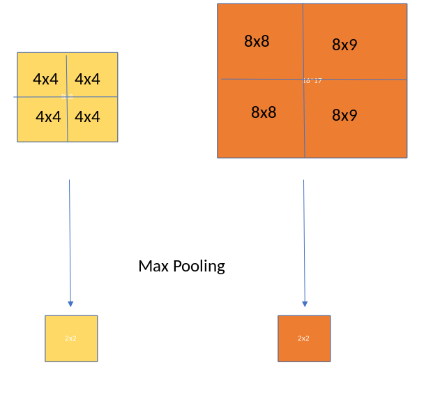
ROI Pooling 2x2

从前面的部分我们可以得到 gt_roi_locs, gt_roi_labels 和 sample_rois. 我们将会使用 sample_rois 作为 roi_pooling层的输入. 注意 sample_rois的规格是 [N, 4] ，每行的格式是 yxhw [y, x, h, w]. 我们需要对这书组做两个改变：

• 添加图像的索引[这里我们只有一个图像]

• 将格式改为xywh

因为sample_rois是一个 numpy数组,我们将会转换为Pytorch张量. 创建roi_indices 张量：

rois = torch.from_numpy(sample_rois).float()
roi_indices = 0 * np.ones((len(rois),), dtype=np.int32)
roi_indices = torch.from_numpy(roi_indices).float()
print(rois.shape, roi_indices.shape)
#Out:
#torch.Size([128, 4]) torch.Size([128])

合并 rois and roi_indices, 这样我们将会得到维度是[N, 5] (index, x, y, h, w)的张量：

indices_and_rois = torch.cat([roi_indices[:, None], rois], dim=1)
xy_indices_and_rois = indices_and_rois[:, [0, 2, 1, 4, 3]]
indices_and_rois = xy_indices_and_rois.contiguous()
print(xy_indices_and_rois.shape)
#Out:
#torch.Size([128, 5])

现在我们需要将数组传到roi_pooling层。我们将会简短的讨论它的作用，解释如下：

- Multiply the dimensions of rois with the sub_sampling ratio (16 in this case)
- Empty output Tensor
- Take each roi
    - subset the feature map based on the roi dimension
    - Apply AdaptiveMaxPool2d to this subset Tensor.
    - Add the outputs to the output Tensor
- Empty output Tensor goes to the network

我们将会定义这个大小为 7 x 7和定义adaptive_max_pool：

size = (7, 7)
adaptive_max_pool = AdaptiveMaxPool2d(size[0], size[1])
output = []
rois = indices_and_rois.data.float()
rois[:, 1:].mul_(1/16.0) # Subsampling ratio
rois = rois.long()
num_rois = rois.size(0)
for i in range(num_rois):
    roi = rois[i]
    im_idx = roi[0]
    im = out_map.narrow(0, im_idx, 1)[..., roi[2]:(roi[4]+1), roi[1]:(roi[3]+1)]
    output.append(adaptive_max_pool(im))

output = torch.cat(output, 0)
print(output.size())
#Out:
# torch.Size([128, 512, 7, 7])
# Reshape the tensor so that we can pass it through the feed forward layer.
k = output.view(output.size(0), -1)
print(k.shape)

#Out:
# torch.Size([128, 25088])

现在这将会是一个classifier层的输入, 进一步将会如同下面图表所示的分出classification head 和 regression head 。 现在让我们定义网络：

roi_head_classifier = nn.Sequential(*[nn.Linear(25088, 4096),
                                      nn.Linear(4096, 4096)])
cls_loc = nn.Linear(4096, 21 * 4) # (VOC 20 classes + 1 background. Each wil

cls_loc.weight.data.normal_(0, 0.01)
cls_loc.bias.data.zero_()
score = nn.Linear(4096, 21) # (VOC 20 classes + 1 background)

将roi-pooling的输出传到上面我们定义的网络：

k = roi_head_classifier(k)
roi_cls_loc = cls_loc(k)
roi_cls_score = score(k)
print(roi_cls_loc.shape, roi_cls_score.shape)
#Out:
# torch.Size([128, 84]), torch.Size([128, 21])

roi_cls_loc 和 roi_cls_score 是从实际边界区域得到的两个输出张量，我们将会在第8部分看到这部分内容。在第7部分，我们将会计算关于 RPN 和 Fast RCNN 网络的损失。这将会完整了Faster R-CNN的实现。

  损失函数

我们有两种网络，RPN和Fast-RCNN，相对应的特征就会有两种输出（Regression头和 classification头）。对于这两种网络的损失函数如下：

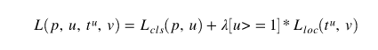
Faster RCNN 损失

  RPN损失

RPN损失

在这里p_{i}是预测类标签， p_{i}^*是实际类数值。t_{i} 和 t_{i}^* 是预测坐标和实际坐标。如果anchor是正的，则实况标签p_{i}^*为1，否则为0。我们将会看到如何在Pytorch中实现。

在第2部分，我们计算了Anchor box的目标值，在第3部分我们计算了RPN网络的输出值。两者的差值将会给出RPN损失。我们将会看到如何计算。

print(pred_anchor_locs.shape)
print(pred_cls_scores.shape)
print(anchor_locations.shape)
print(anchor_labels.shape)
#Out:
# torch.Size([1, 12321, 4])
# torch.Size([1, 12321, 2])
# (12321, 4)
# (12321,)

我们将会从新排列，将输入和输出排成一行：

rpn_loc = pred_anchor_locs[0]
rpn_score = pred_cls_scores[0]
gt_rpn_loc = torch.from_numpy(anchor_locations)
gt_rpn_score = torch.from_numpy(anchor_labels)
print(rpn_loc.shape, rpn_score.shape, gt_rpn_loc.shape, gt_rpn_score.shape)
#Out
# torch.Size([12321, 4]) torch.Size([12321, 2]) torch.Size([12321, 4])

pred_cls_scores 和 anchor_labels 是RPN网络的预测对象值和实际对象值。我们将会用如下的分别对于Regression and classification 的损失函数。

对与classification我们使用Cross Entropy损失：

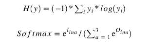
Cross Entropy 损失

使用Pytorch我们可以计算损失：

import torch.nn.functional as F
rpn_cls_loss = F.cross_entropy(rpn_score, gt_rpn_score.long(), ignore_index = -1)
print(rpn_cls_loss)

#Out:
# Variable containing:
#  0.6940
# [torch.FloatTensor of size 1]

对于 Regression 我们使用smooth L1 损失，如在Fast RCNN 论文中定义的：

Smooth L1损失 

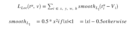
使用 L1 而不是 L2 损失，是因为RPN的预测回归头的值不是有限的。 Regression 损失也被应用在有正标签的边界区域中：

pos = gt_rpn_score > 0
mask = pos.unsqueeze(1).expand_as(rpn_loc)
print(mask.shape)
#Out:
# torch.Size(12321, 4)

现在取有正数标签的边界区域：

mask_loc_preds = rpn_loc[mask].view(-1, 4)
mask_loc_targets = gt_rpn_loc[mask].view(-1, 4)
print(mask_loc_preds.shape, mask_loc_preds.shape)
#Out:
# torch.Size([6, 4]) torch.Size([6, 4])

regression损失应用如下 ：

x = torch.abs(mask_loc_targets - mask_loc_preds)
rpn_loc_loss = ((x < 1).float() * 0.5 * x**2) + ((x >= 1).float() * (x-0.5))
print(rpn_loc_loss.sum())
#Out:
# Variable containing:
#  0.3826
# [torch.FloatTensor of size 1]

合并rpn_cls_loss 和 rpn_reg_loss, 因为class loss 应用在全部的边界区域，regression loss 应用在正数标签边界区域,作者已经介绍  Λ 作为超参数。通过使用边界区域的数量：

rpn_lambda = 10.
N_reg = (gt_rpn_score >0).float().sum()
rpn_loc_loss = rpn_loc_loss.sum() / N_reg
rpn_loss = rpn_cls_loss + (rpn_lambda * rpn_loc_loss)
print(rpn_loss)
#Out:0.00248

  Fast R-CNN 损失函数

快速的R-CNN损失函数也以同样的方式实现，几乎没有调整。

我们有下列的变量：

1.预测：

print(roi_cls_loc.shape)
print(roi_cls_score.shape)
#Out:
# torch.Size([128, 84])
# torch.Size([128, 21])

2.真实：

print(gt_roi_locs.shape)
print(gt_roi_labels.shape)
#Out:
#(128, 4)
#(128, )

3.转化金标准到Torch变量：

gt_roi_loc = torch.from_numpy(gt_roi_locs)
gt_roi_label = torch.from_numpy(np.float32(gt_roi_labels)).long()
print(gt_roi_loc.shape, gt_roi_label.shape)

#Out:
#torch.Size([128, 4]) torch.Size([128])

4.分类损失：

roi_clss_loss = F.cross_entropy(roi_cls_score, rt_roi_label, ignore_index=-1)
print(roi_cls_loss.shape)
#Out:
#Variable containing:
#  3.0458
# [torch.FloatTensor of size 1]

5.回归损失对于回归损失，每个ROI位置有21（num_classes+background）预测边界框。为了计算损失，我们将只使用带有正标签的边界框（P_i^*）：

n_sample = roi_cls_loc.shape[0]
roi_loc = roi_cls_loc.view(n_sample, -1, 4)
print(roi_loc.shape)
#Out:
#torch.Size([128, 21, 4])
roi_loc = roi_loc[torch.arange(0, n_sample).long(), gt_roi_label]
print(roi_loc.shape)
#Out:
#torch.Size([128, 4])

用计算RPN网络回归损失的方法计算回归损失，我们得到：

roi_loc_loss = REGLoss(roi_loc, gt_roi_loc)
print(roi_loc_loss)

#Out:
#Variable containing:
#  0.1895
# [torch.FloatTensor of size 1]

注意，我们这里没有写任何regloss函数。读者可以包装在RPN Reg Loss中讨论的所有方法，并实现这个函数。

6.ROI损失总和

损失总和：

roi_lambda = 10.
roi_loss = roi_cls_loss + (roi_lambda * roi_loc_loss)
print(roi_loss)

#Out:
#Variable containing:
#  4.2353
# [torch.FloatTensor of size 1]

损失总和：

现在我们需要结合RPN损失和快速RCNN损失来计算1次迭代的总sunshi。这是一个简单的添加。

total_loss = rpn_loss + roi_loss

就是这样，我们必须在训练过程中通过一张接着一张的图像重复多次。

就是这样。更快的RCNN论文讨论了这种神经网络的不同训练方法。可参阅参考资料一节中的论文。

  注意要点：

• Faster RCNN是通过特征金字塔网络（FPN）进行改善的，anchor box的数量大概接近于100000，在鉴定小的对象上更精确

• Faster RCNN更多的使用Resnet和ResNext这类进行训练

• Faster RCNN是对于实例分割来说最先进的单一模型mask-rcnn的主干模型

  参考文献

• https://arxiv.org/abs/1506.01497

• https://github.com/chenyuntc/simple-faster-rcnn-pytorch

作者：Prakashjay. 贡献： Suraj Amonkar, Sachin Chandra, Rajneesh Kumar 和 Vikash Challa.

多谢您的阅读，学习愉快。

想要继续查看该篇文章相关链接和参考文献？

长按链接点击打开或点击底部【阅读原文】：

https://ai.yanxishe.com/page/TextTranslation/1304

AI研习社每日更新精彩内容，观看更多精彩内容：

盘点图像分类的窍门

深度学习目标检测算法综述

生成模型：基于单张图片找到物体位置

AutoML :无人驾驶机器学习模型设计自动化

等你来译：

如何在神经NLP处理中引用语义结构 

你睡着了吗？不如起来给你的睡眠分个类吧！ 

高级DQNs：利用深度强化学习玩吃豆人游戏

深度强化学习新趋势：谷歌如何把好奇心引入强化学习智能体 

春

节

挑

战

2月2日至2月12日，AI求职百题斩之每日挑战限时升级，赶紧来答题吧！

0207期  答题须知

请在公众号菜单【每日一题】→【每日一题】进入，或发送【0207】即可答题并获取解析。

点击阅读原文，查看更多内容