神经网络编程 - 前向传播和后向传播（附完整代码）- 专知

神经网络编程 - 前向传播和后向传播（附完整代码）

【导读】本文的目的是深入分析深层神经网络，剖析神经网络的结构，并在此基础上解释重要概念，具体分为两部分：神经网络编程和应用。在神经网络编程部分，讲解了前向传播和反向传播的细节，包括初始化参数、激活函数、损失函数等。在应用部分，通过一个图像分类实例讲解如何一步步构建神经网络。

作者 | Imad Dabbura

编译 | 专知

参与 | Yingying, Xiaowen

神经网络编程 - 前向传播和后向传播

根据无限逼近定理（Universal approximation theorem），神经网络可以在有限的层数和误差范围内学习和表示任何函数。神经网络学习真实函数的方法是在简单表示的基础上建立复杂的表示。在每个隐藏层上，神经网络首先计算给定输入的线性变换，然后应用非线性函数，而后者将成为下一层的输入，从而学习新的特征，直到输出层。因此，我们可以将神经网络定义为信息从输入通过隐藏层流向输出。

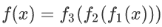
对于3层神经网络，学习函数为：

其中：

：在第一个隐藏层学习的函数

：在第二个隐藏层学习的函数

：在输出层学习的函数

因此，在每一层上，我们学习的是不同的表示方式，这些表示方式会随着隐藏层层数变多而变得更加复杂。下面是一个3层神经网络的例子（我们不考虑输入层）：

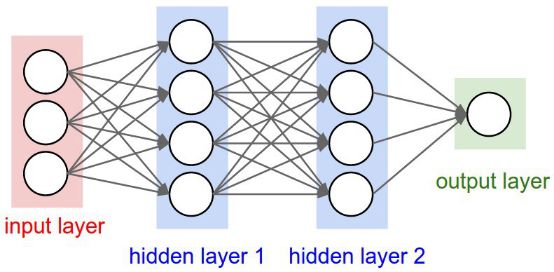
例如，计算机无法直接理解图像，也不知道如何处理像素。然而，神经网络可以在前面的隐藏层中建立一个简单的图像表示来识别边缘，通过第一个隐藏层，它可以学习角点和轮廓，通过第二个隐藏层，它可以学习诸如鼻子等部分。最后，它可以学习对象整体。

表示对于机器学习算法的性能非常关键，神经网络可以帮助我们构建非常复杂的模型，并将其留给算法来学习这样的表示，而不用担心花很长时间进行特征工程。

这个博客分为两部分：

1. 神经网络编程：这需要编写所有帮助我们实现多层神经网络的帮助函数。

2. 应用：我们将在第一部分中对图像识别问题编码的神经网络进行实现，以查看我们构建的网络是否能够检测到图像是否有猫或狗。

第一步是引入相应的包

# Import packages
import h5py import
matplotlib.pyplot as plt
import numpy as np
import seaborn as sns

神经网络编程

前向传播

输入X提供初始信息，然后传播到每层的隐藏单元，最后输出。网络的体系结构确定了层数和每层节点数和激活函数。有很多激活函数，如整流线性单元，Sigmoid，双曲正切等等。研究已经证明，深层网络胜过拥有更多隐藏单元的网络。因此，训练更深层次的网络（收益递减）总是会更好。

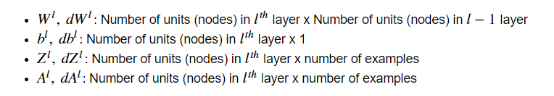
让我们先介绍一下在整个帖子中使用的一些符号：

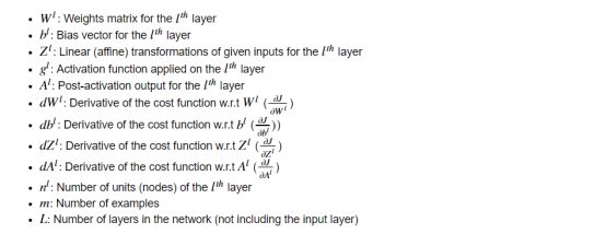
接下来，我们将以一般形式写下多层神经网络的维度，以帮助我们进行矩阵乘法，因为实现神经网络的主要挑战之一是使维度正确。

初始化参数

我们首先初始化权重矩阵和偏置向量。要注意，我们不应该将所有参数初始化为零，因为这样做会导致梯度相等，并且在每次迭代时输出都是相同的，且学习算法不会学到任何东西。因此，将参数随机初始化为0到1之间的值非常重要。建议将随机值乘以小标量（例如0.01），以使激活单元处于活动状态，并位于激活函数的导数不接近于零的区域。

# Initialize parameters
def initialize_parameters(layers_dims):
    np.random.seed(1)
    parameters = {}
    L = len(layers_dims)
    for l in range(1, L):
        parameters["W" + str(l)] = np.random.randn( layers_dims[l], layers_dims[l - 1]) *
         0.01
        parameters["b" + str(l)] = np.zeros((layers_dims[l], 1))
        assert parameters["W" + str(l)].shape == ( layers_dims[l], layers_dims[l - 1])
        assert parameters["b" + str(l)].shape == (layers_dims[l], 1)
        return parameters

激活函数

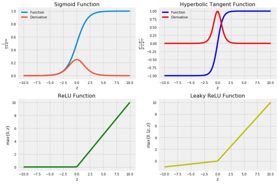
没有关于哪个激活函数最适用于某个特定问题的明确说明。这是一个尝试错误的过程，在这个过程中，人们应该尝试不同的函数，并且看看哪一个函数对于手头的问题最有效。我们将涵盖4个最常用的激活函数：

Sigmoid函数（σ）：建议仅在输出层使用，以便我们可以轻松地将输出解释为概率，因为它将输出限制在0和1之间。在其大部分域上梯度非常接近于零，这使得学习算法学习速度慢，难度大。
双曲正切函数：。它优于sigmoid函数，其中输出的平均值非常接近于零，换句话说，激活单元的输出集中在零点附近，使值的范围非常小，这意味着学习速度更快。它与Sigmoid函数的缺点都是在域的很大一部分上梯度很小。
修正线性单元（ReLU）：接近线性的模型很容易优化。由于ReLU拥有很多线性函数的特性，因此它在大多数问题上都可以很好地工作。唯一的问题是导数没有在z = 0处定义，我们可以通过在z = 0处将导数赋值为0来克服。但是，这意味着对于z≤0，梯度为零而且也不能学习。
leaky修正线性单元（Leaky Rectibed Linear Unit）：它克服了来自ReLU的零梯度问题，并为z≤0分配了一个小值α。

如果您不确定要选择哪个激活函数，请从ReLU开始。接下来，我们将实现上述激活函数并可视化，以便更容易地看到每个函数的域和范围。

# Define activation functions that will be used in forward propagation
def sigmoid(Z):
    A = 1 / (1 + np.exp(-Z))
    return A, Z

def tanh(Z):
    A = np.tanh(Z)
    return A, Z

def relu(Z):
    A = np.maximum(0, Z)
    return A, Z

def leaky_relu(Z):
    A = np.maximum(0.1 * Z, Z)
    return A, Z

# Plot the 4 activation functions
z = np.linspace(-10, 10, 100)
# Computes post-activation outputs
A_sigmoid, z = sigmoid(z)
A_tanh, z = tanh(z)
A_relu, z = relu(z)
A_leaky_relu, z = leaky_relu(z)
# Plot sigmoid
plt.figure(figsize=(12, 8))
plt.subplot(2, 2, 1)
plt.plot(z, A_sigmoid, label = "Function")
plt.plot(z, A_sigmoid * (1 - A_sigmoid), label = "Derivative") 
plt.legend(loc = "upper left")
plt.xlabel("z")
plt.ylabel(r"$\frac{1}{1 + e^{-z}}$")
plt.title("Sigmoid Function", fontsize = 16)
# Plot tanh
plt.subplot(2, 2, 2)
plt.plot(z, A_tanh, 'b', label = "Function")
plt.plot(z, 1 - np.square(A_tanh), 'r',label = "Derivative") 
plt.legend(loc = "upper left")
plt.xlabel("z")
plt.ylabel(r"$\frac{e^z - e^{-z}}{e^z + e^{-z}}$") 
plt.title("Hyperbolic Tangent Function", fontsize = 16)
# plot relu
plt.subplot(2, 2, 3)
plt.plot(z, A_relu, 'g')
plt.xlabel("z")
plt.ylabel(r"$max\{0, z\}$")
plt.title("ReLU Function", fontsize = 16)
# plot leaky relu
plt.subplot(2, 2, 4)
plt.plot(z, A_leaky_relu, 'y')
plt.xlabel("z")
plt.ylabel(r"$max\{0.1z, z\}$")
plt.title("Leaky ReLU Function", fontsize = 16)
plt.tight_layout();

前馈

给定其来自前一层的输入，每个单元计算仿射变换，然后应用激活函数。在这个过程中，我们将存储（缓存）每个层上计算和使用的所有变量，以用于反向传播。我们将编写前两个辅助函数，这些函数将用于L模型向前传播，以便于调试。请记住，在每一层，我们可能有不同的激活函数。

# Define helper functions that will be used in L-model forward prop 
def linear_forward(A_prev, W, b):
    Z = np.dot(W, A_prev) + b
    cache = (A_prev, W, b)
    return Z, cache

def linear_activation_forward(A_prev, W, b, activation_fn):
    assert activation_fn == "sigmoid" or activation_fn == "tanh" 
or \ activation_fn == "relu"
    if activation_fn == "sigmoid":
        Z, linear_cache = linear_forward(A_prev, W, b)
        A, activation_cache = sigmoid(Z)
    elif activation_fn == "tanh":
        Z, linear_cache = linear_forward(A_prev, W, b)
        A, activation_cache = tanh(Z)
    elif activation_fn == "relu":
        Z, linear_cache = linear_forward(A_prev, W, b)
        A, activation_cache = relu(Z)
    assert A.shape == (W.shape[0], A_prev.shape[1])
    cache = (linear_cache, activation_cache)
    return A, cache

def L_model_forward(X, parameters, hidden_layers_activation_fn="relu"):
    A = X caches = []   
    L = len(parameters) // 2
    for l in range(1, L):
        A_prev = A
        A, cache = linear_activation_forward( A_prev, parameters["W" + str(l)], 
parameters["b" + str(l)], activation_fn=hidden_layers_activation_fn)
        caches.append(cache)
        AL, cache = linear_activation_forward( A, parameters["W" + str(L)], 
parameters["b" + str(L)], activation_fn="sigmoid")
        caches.append(cache)
    assert AL.shape == (1, X.shape[1])
    return AL, caches

损失

我们将使用二元交叉熵损失函数。它使用对数似然方法来估计误差。损失是：上述损失函数是凸的; 然而，神经网络通常停留在局部最小值，并不能保证找到最佳参数。我们将在这里使用基于梯度的学习算法。

# Compute cross-entropy cost
def compute_cost(AL, y):
    m = y.shape[1]
    cost = - (1 / m) * np.sum( np.multiply(y, np.log(AL)) + 
    np.multiply(1 - y, np.log(1 - AL)))
    return cost

反向传播

通过网络允许信息从损失中返回，以计算梯度。因此，误差从最后的输出节点传到开始的节点，来计算关于每个边的节点相对于的最终节点输出的导数。这样做可以帮助我们知道谁导致了大的误差，并在这个方向上改变参数。

# Define derivative of activation functions w.r.t z that will be used in back-propagation 
def sigmoid_gradient(dA, Z):
    A, Z = sigmoid(Z)
    dZ = dA * A * (1 - A)
    return dZ


def tanh_gradient(dA, Z):
    A, Z = tanh(Z)
    dZ = dA * (1 - np.square(A))
    return dZ


def relu_gradient(dA, Z):
    A, Z = relu(Z)
    dZ = np.multiply(dA, np.int64(A > 0))
    return dZ


# define helper functions that will be used in L-model back-prop 
def linear_backword(dZ, cache):
    A_prev, W, b = cache
    m = A_prev.shape[1]
    dW = (1 / m) * np.dot(dZ, A_prev.T)
    db = (1 / m) * np.sum(dZ, axis=1, keepdims=True)
    dA_prev = np.dot(W.T, dZ)
    assert dA_prev.shape == A_prev.shape
    assert dW.shape == W.shape
    assert db.shape == b.shape
    return dA_prev, dW, db


def linear_activation_backward(dA, cache, activation_fn):
    linear_cache, activation_cache = cache
    if activation_fn == "sigmoid":
        dZ = sigmoid_gradient(dA, activation_cache)
        dA_prev, dW, db = linear_backword(dZ, linear_cache)
    elif activation_fn == "tanh":
        dZ = tanh_gradient(dA, activation_cache)
        dA_prev, dW, db = linear_backword(dZ, linear_cache)
    elif activation_fn == "relu":
        dZ = relu_gradient(dA, activation_cache)
        dA_prev, dW, db = linear_backword(dZ, linear_cache)
    return dA_prev, dW, db


def L_model_backward(AL, y, caches, hidden_layers_activation_fn="relu"):
    y = y.reshape(AL.shape)
    L = len(caches)
    grads = {}
    dAL = np.divide(AL - y, np.multiply(AL, 1 - AL))
    grads["dA" + str(L - 1)], grads["dW" + str(L)], grads["db" + str(L)] = 
    linear_activation_backward(dAL, caches[L - 1],"sigmoid")
    for l in range(L - 1, 0, -1):
        current_cache = caches[l - 1]
        grads["dA" + str(l - 1)], grads["dW" + str(l)], grads["db" + str(l)] = 
        linear_activation_backward(
            grads["dA" + str(l)], current_cache, hidden_layers_activation_fn)
        return grads

    # define the function to update both weight matrices and bias vectors 


def update_parameters(parameters, grads, learning_rate): L = len(parameters) // 2


for l in range(1, L + 1):
    parameters["W" + str(l)] = parameters["W" + str(l)] - 
    learning_rate * grads["dW" + str(l)]
    parameters["b" + str(l)] = parameters["b" + str(l)] - 
    learning_rate * grads["db" + str(l)]
return parameters

应用

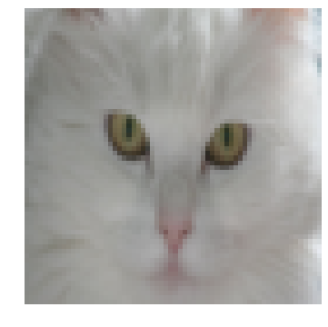
我们将处理209张图像的数据集。每个图像分辨率为64*64。我们建立一个神经网络来分类图像是否有猫。因此，。

我们首先加载图像。
显示猫的示例图像。
重塑输入矩阵，以便每列都是一个样例。此外，由于每张图片都是64 x 64 x 3，因此每张图片最终都会有12,288个特征。因此，输入矩阵将是12,288 x 209。
标准化数据使梯度不会失控。此外，这将有助于隐藏单元都具有相似的值的范围。然后我们将每个像素除以255。但是最好将数据标准化为平均值为0，标准差为1。

# Import training dataset
train_dataset = h5py.File("../data/train_catvnoncat.h5")
X_train = np.array(train_dataset["train_set_x"])
y_train = np.array(train_dataset["train_set_y"])
test_dataset = h5py.File("../data/test_catvnoncat.h5")
X_test = np.array(test_dataset["test_set_x"])
y_test = np.array(test_dataset["test_set_y"])
# print the shape of input data and label vector
print(f"""Original dimensions:\n{20 * '-'}\nTraining: {X_train.shape}, 
{y_train.shape} Test: {X_test.shape}, {y_test.shape}""")
# plot cat image
plt.figure(figsize=(6, 6))
plt.imshow(X_train[50])
plt.axis("off");
# Transform input data and label vector
X_train = X_train.reshape(209, -1).T
y_train = y_train.reshape(-1, 209)
X_test = X_test.reshape(50, -1).T
y_test = y_test.reshape(-1, 50)
# standarize the data
X_train = X_train / 255
X_test = X_test / 255
print(f"""\nNew dimensions:\n{15 * '-'}\nTraining: {X_train.shape}, 
{y_train.shape} Test: {X_test.shape}, {y_test.shape}""")
Original dimensions:
--------------------
Training: (209, 64, 64, 3), (209,)
Test: (50, 64, 64, 3), (50,)
New dimensions:
---------------
Training: (12288, 209), (1, 209)
Test: (12288, 50), (1, 50)

现在，数据集已经准备好了。我们首先编写多层模型函数，使用预定义的迭代次数和学习率来实现基于梯度的学习。

# Define the multi-layer model using all the helper functions we wrote before
def L_layer_model( X, y, layers_dims, learning_rate=0.01, num_iterations=3000, 
print_cost=True, hidden_layers_activation_fn="relu"):
np.random.seed(1)
# initialize parameters
parameters = initialize_parameters(layers_dims)
# intialize cost list
cost_list = []
# iterate over num_iterations
for i in range(num_iterations):
# iterate over L-layers to get the final output and the cache
AL, caches = L_model_forward( X, parameters, hidden_layers_activation_fn)
# compute cost to plot it
cost = compute_cost(AL, y)
# iterate over L-layers backward to get gradients
grads = L_model_backward(AL, y, caches, hidden_layers_activation_fn) 
# update parameters
parameters = update_parameters(parameters, grads, learning_rate)
# append each 100th cost to the cost list
if (i + 1) % 100 == 0 and print_cost:
print(f"The cost after {i + 1} iterations is: {cost:.4f}")
if i % 100 == 0:
cost_list.append(cost)
# plot the cost curve
plt.figure(figsize=(10, 6))
plt.plot(cost_list)
plt.xlabel("Iterations (per hundreds)")
plt.ylabel("Loss")
plt.title(f"Loss curve for the learning rate = {learning_rate}") return parameters
def accuracy(X, parameters, y, activation_fn="relu"):
probs, caches = L_model_forward(X, parameters, activation_fn)
labels = (probs >= 0.5) * 1
accuracy = np.mean(labels == y) * 100
return f"The accuracy rate is: {accuracy:.2f}%."

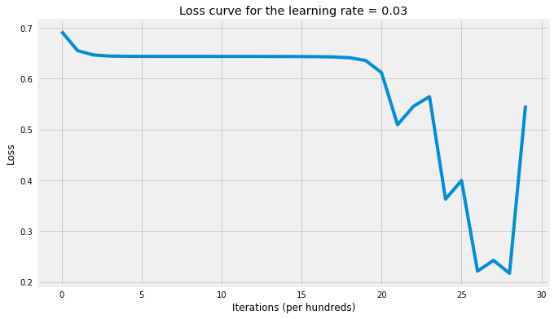
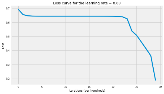
接下来，我们将训练两个神经网络的版本，每个版本将在隐藏层上使用不同的激活函数：一个将使用修正线性单元（ReLU），另一个将使用双曲正切函数（tanh）。最后，我们将使用我们从两个神经网络获得的参数对训练样例进行分类并计算每个版本的训练准确率，来发现哪个激活函数在这个问题上最有效。

# Setting layers dims
layers_dims = [X_train.shape[0], 5, 5, 1]
# NN with tanh activation fn
parameters_tanh = L_layer_model( X_train, y_train, layers_dims, learning_rate=0.03, 
num_iterations=3000, hidden_layers_activation_fn="tanh")
# Print the accuracy
accuracy(X_test, parameters_tanh, y_test, activation_fn="tanh")
The cost after 100 iterations is: 0.6556 
The cost after 200 iterations is: 0.6468
The cost after 300 iterations is: 0.6447
The cost after 400 iterations is: 0.6441
The cost after 500 iterations is: 0.6440
The cost after 600 iterations is: 0.6440
The cost after 700 iterations is: 0.6440
The cost after 800 iterations is: 0.6439
The cost after 900 iterations is: 0.6439
The cost after 1000 iterations is: 0.6439
The cost after 1100 iterations is: 0.6439
The cost after 1200 iterations is: 0.6439
The cost after 1300 iterations is: 0.6438
The cost after 1400 iterations is: 0.6438
The cost after 1500 iterations is: 0.6437
The cost after 1600 iterations is: 0.6434
The cost after 1700 iterations is: 0.6429
The cost after 1800 iterations is: 0.6413
The cost after 1900 iterations is: 0.6361
The cost after 2000 iterations is: 0.6124
The cost after 2100 iterations is: 0.5112
The cost after 2200 iterations is: 0.5288
The cost after 2300 iterations is: 0.4312
The cost after 2400 iterations is: 0.3821
The cost after 2500 iterations is: 0.3387
The cost after 2600 iterations is: 0.2349
The cost after 2700 iterations is: 0.2206
The cost after 2800 iterations is: 0.1927
The cost after 2900 iterations is: 0.4669
The cost after 3000 iterations is: 0.1040 
'The accuracy rate is: 68.00%.'

# NN with relu activation fn
parameters_relu = L_layer_model( X_train, y_train, layers_dims, learning_rate=0.03, 
num_iterations=3000, hidden_layers_activation_fn="relu")
# Print the accuracy
accuracy(X_test, parameters_relu, y_test, activation_fn="relu")
The cost after 100 iterations is: 0.6556
The cost after 200 iterations is: 0.6468
The cost after 300 iterations is: 0.6447
The cost after 400 iterations is: 0.6441
The cost after 500 iterations is: 0.6440
The cost after 600 iterations is: 0.6440 
The cost after 700 iterations is: 0.6440 
The cost after 800 iterations is: 0.6440 
The cost after 900 iterations is: 0.6440 
The cost after 1000 iterations is: 0.6440 
The cost after 1100 iterations is: 0.6439 
The cost after 1200 iterations is: 0.6439 
The cost after 1300 iterations is: 0.6439 
The cost after 1400 iterations is: 0.6439 
The cost after 1500 iterations is: 0.6439 
The cost after 1600 iterations is: 0.6439 
The cost after 1700 iterations is: 0.6438 
The cost after 1800 iterations is: 0.6437 
The cost after 1900 iterations is: 0.6435 
The cost after 2000 iterations is: 0.6432 
The cost after 2100 iterations is: 0.6423 
The cost after 2200 iterations is: 0.6395 
The cost after 2300 iterations is: 0.6259 
The cost after 2400 iterations is: 0.5408 
The cost after 2500 iterations is: 0.5262 
The cost after 2600 iterations is: 0.4727 
The cost after 2700 iterations is: 0.4386 
The cost after 2800 iterations is: 0.3493 
The cost after 2900 iterations is: 0.1877 
The cost after 3000 iterations is: 0.3641
'The accuracy rate is: 42.00%.'

请注意，上述准确率预计会高估泛化准确率。

结论

这篇文章的目的是深入分析深层神经网络，并在此基础上解释重要概念。我们现在并不关心准确率，因为我们可以做很多事情来提高准确性，这将是以下帖子的主题。以下是一些要点：

即使神经网络可以表示任何函数，但由于两个原因可能会失败：
1. 优化算法可能无法找到所需（真）函数参数的最佳值。它可以陷入局部最佳状态。
2. 由于过拟合，学习算法可能会找到与预期函数不同的形式。
即使神经网络很难收敛并总是陷入局部最小值，它仍然能够显著降低损失，并且提出测试精度高的非常复杂的模型。
我们在这篇文章中使用的神经网络是标准的全连接网络。但是，还有另外两种网络：
1. CNN：不是所有节点都进行连接。这是图像识别最好的模型。
2. RNN：反馈连接将模型的输出反馈到自身。它主要用于顺序建模。
全连接神经网络也忘记了以前的步骤发生了什么，也不知道输出的任何信息。
我们可以使用交叉验证来调整多个超参数，以获得网络的最佳性能：
1. 学习率（α）：确定每次更新参数的步数。
A. 过小的α会导致收敛速度缓慢，并可能在计算上非常昂贵。
B. 过大的α可能导致过冲，因为我们的学习算法可能永远不会收敛。
2. 隐藏层的数量（深度）：隐藏层越多越好，但是计算成本高。
3. 每个隐藏层的单元数量（宽度）：研究证明，每层隐藏单元的数量并不会改进网络。
4. 激活函数：在隐藏层上使用的函数在应用和域之间是不同的。尝试不同的函数并查看哪种功能最有效是一个尝试和错误的过程。
5. 迭代次数：
标准化数据将有助于激活单位具有相似的数值范围并避免梯度爆炸或消失。