[专知-Java Deeplearning4j 深度学习教程 04] 使用 CNN 进行文本分类:图文-代码
【导读】主题链路知识是我们专知的核心功能之一,为用户提供AI领域系统性的知识学习服务,一站式学习人工智能的知识,包含人工智能( 机器学习、自然语言处理、计算机视觉等)、大数据、编程语言、系统架构。使用请访问专知 进行主题搜索查看 - 桌面电脑访问http://www.zhuanzhi.ai, 手机端访问http://www.zhuanzhi.ai 或关注微信公众号后台回复" 专知"进入专知,搜索主题查看。继Pytorch教程后,我们推出面向Java程序员的深度学习教程DeepLearning4J。Deeplearning4j的案例和资料很少,官方的doc文件也非常简陋,基本上所有的类和函数的都没有解释。为此,我们推出来自中科院自动化所专知小组博士生Hujun与Sanglei创作的-分布式Java开源深度学习框架Deeplearning4j学习教程包括以下:
- 【专知-Java Deeplearning4j深度学习教程01】分布式Java开源深度学习框架DL4j安装使用: 图文+代码
- 【专知-Java Deeplearning4j深度学习教程02】用ND4J自己动手实现RBM: 图文+代码
- 【专知-Java Deeplearning4j深度学习教程03】使用多层神经网络分类MNIST数据集:图文+代码
- 【专知-Java Deeplearning4j深度学习教程04】使用CNN进行文本分类:图文+代码
- 【专知-Java Deeplearning4j深度学习教程05】无监督特征提取神器—AutoEncoder:图文+代码
- 【专知-Java Deeplearning4j深度学习教程06】用卷积神经网络CNN进行图像分类
简介
卷积神经网络(Convolutional Neural Network, CNN), 最早应用在图像处理领域。从最早的mnist手写体数字识别,到ImageNet大规模图像分类比赛,再到炙手可热的自动驾驶技术,CNN在其中都起到了举足轻重的作用。
最近CNN也被成功的应用到自然语言处理领域(Natural Language Processing),并取得了引人注目的成果。我将在本文中归纳什么是CNN,并以一个简单的文本分类的例子介绍怎样将CNN应用于NLP。CNN背后的直觉知识在计算机视觉的用例里更容易被理解,因此我就先从那里开始,然后慢慢过渡到自然语言处理。
什么是卷积运算
卷积神经网络与之前讲到的常规的神经网络非常相似:它们都是由神经元组成,神经元中有具有学习能力的权重和偏差。每个神经元都得到一些输入数据,进行内积运算后再进行激活函数运算。
那么有哪些地方变化了呢?卷积神经网络的结构基于一个假设,即输入数据是二维的图像,基于该假设,我们就向结构中添加了一些特有的性质。这些特有属性使得前向传播函数实现起来更高效,并且大幅度降低了网络中参数的数量。
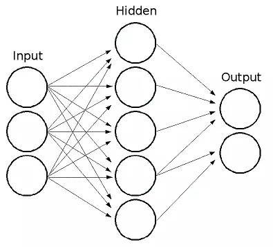
上图是常规的全连接网络,我们可以看到这里的输入层就是一维向量,后续的处理方式使用简单的全连接层就可以了。而卷积网络的输入要求是二维向量,这就需要向网络结构中加入一些新的特性来处理,也就是卷积操作
http://deeplearning.stanford.edu/wiki/index.php/Feature_extraction_using_convolution
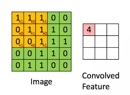
图中绿色为一个二值图像,每个值代表一个像素(0是黑,1是白)。(更典型的是像素值为0-255的灰阶图像)
图中黄色的滑动窗口叫卷积核、过滤器或者特征检测器,也是一个矩阵。
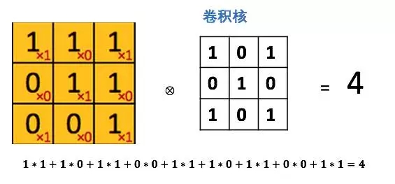
将这个大小是3x3的过滤器中的每个元素(红色小字)与图像中对应位置的值相乘,然后对它们求和,得到右边粉红色特征图矩阵的第一个元素值。
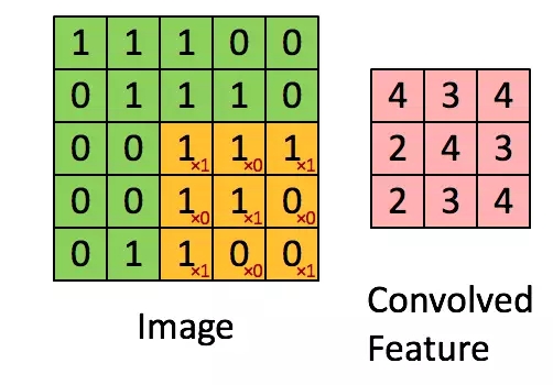
在整个图像矩阵上滑动这个过滤器来得到完整的卷积特征图如下:
什么是卷积神经网络?
知道了卷积运算了吧。那CNN又是什么呢?CNN本质上就是多层卷积运算,外加对每层的输出用非线性激活函数做转换,比如用ReLU和tanh。
常规的神经网络把每个输入神经元与下一层的输出神经元相连接。这种方式也被称作是全连接层。
在CNN中我们不这样做,而是用输入层的卷积结果来计算输出,也就是上图中的(Convolved Feature)。
这相当于是局部连接,每块局部的输入区域与输出的一个神经元相连接。对每一层应用不同的滤波器,往往是如上图所示成百上千个,然后汇总它们的结果。
这里也涉及到池化层(降采样),我会在后文做解释。
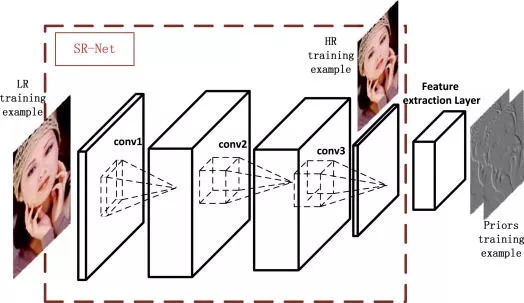
在训练阶段,CNN基于你想完成的任务自动学习卷积核的权重值。
举个例子,在图像分类问题中,第一层CNN模型或许能学会从原始像素点检测到一些边缘线条,然后根据边缘线条在第二层检测出一些简单的形状,然后基于这些形状检测出更高级的特征,比如脸部轮廓等。最后一层是利用这些高级特征的一个分类器。
为什么要用卷积神经网络?
图像处理中,往往会将图像看成是一个或者多个二维向量,传统的神经网络采用全联接的方式,即输入层到隐藏层的神经元都是全部连接的,这样做将导致参数量巨大,使得网络训练耗时甚至难以训练,而CNN则通过局部链接、权值共享等方法避免这一困难。
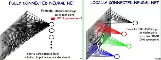
- 局部连接
对于一个1000 ×1000的输入图像而言,如果下一个隐藏层的神经元数目为10^6个,采用全连接则有1000× 1000 × 10^6 =10^12个权值参数,如此数目巨大的参数几乎难以训练;而采用局部连接,假如局部感受野是10x 10,隐藏层的每个神经元仅与图像中10 × 10的局部图像相连接,那么此时的权值参数数量为10 × 10 × 10^6 = 10^8,将直接减少4个数量级。
- 权值共享
隐含层每个神经元都连接10 * 10个图像区域,也就是说每一个神经元存在100个连接权值参数。如果我们每个神经元这100个参数相同呢?将这10×10个权值参数共享给剩下的神经元,也就是说隐藏层中10^6个神经元的权值参数相同,那么此时不管隐藏层神经元的数目是多少,需要训练的参数就是这10 × 10个权值参数(也就是卷积核(也称滤波器)的大小)
这大概就是CNN的一个神奇之处,尽管只有这么少的参数,依旧有出色的性能。但是,这样仅提取了图像的一种特征,如果要多提取出一些特征,可以增加多个卷积核,不同的卷积核能够得到图像的不同映射下的特征,称之为Feature Map。如果有100个卷积核,最终的权值参数也仅为100 × 100 =10^4个而已。另外,偏置参数也是共享的,同一种滤波器共享一个。
感觉好厉害,那如何将CNN用于NLP呢?
要将CNN用到文本处理中首先要解决的就是文本的表示问题。前面提到CNN的输入是一个二维向量,图像的像素表示天然具有这种形式。而对于文本来说,我们通常采用词向量的方法来将一段话表示成二维向量形式。
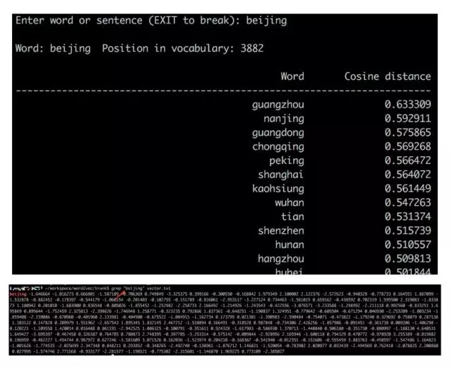
词向量的基本思想是将每个词表示为n维稠密,连续的实数向量,通常是几十到几百维不等。而这些向量表示保存了每个词在语料中出现的一些上下信息,这样我们就可以简单的通过直接计算词表示两个向量的cos距离,来的到他们之间的相似度。现在有很多词向量的学习方式,最具代表性的应该是13年google发表的两篇word2vec,其在随之发布了简单的word2vec工具包,并在语义维度上得到了很好的验证,极大的推动了文本分析的进程。
下边是一个简单的向量相似度计算的例子。与“beijing”这个词的表示向量距离相近的是一些其他的城市名。而“北京”在这里是用一个200维的向量表示的。
在有了每个词的向量表示后,通过简单的拼接将一段文本表示成2维矩阵形式。在这里每一行是一个词的向量表示。
输入是一个句子,为了使其可以进行卷积,首先需要将其转化为向量表示,通常使用word2vec实现。
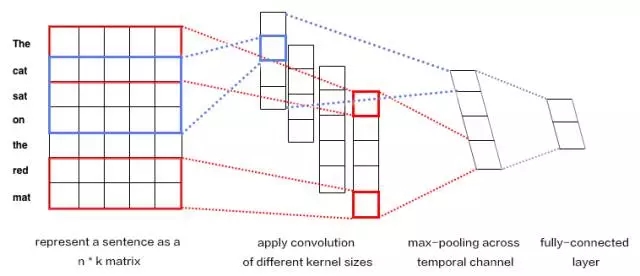
k表示词向量的维度,n是一段文本的长度。文本被表示成[sentence_lengh * word_dimension]的一个二维向量。图中表示为7*5
卷积核每次只对图像的一小块区域运算,但在处理自然语言时滤波器通常覆盖上下几行(几个词)。因此,卷积核的宽度也就和输入矩阵的宽度也就是向量维度相等了。尽管高度,或者区域大小可以随意调整,但一般滑动窗口的覆盖范围是2~5行。
示意图中我们对卷积核设置了2行和3行两种尺寸,每种尺寸各有两种滤波器。的到4个feature map
每个卷积核对句子矩阵做卷积运算,得到(不同程度的)filter。然后对每个filter做最大值池化,也就是只记录filter的最大值。这样,就由4个字典生成了一串单变量特征向量(univariate feature vector)
然后这4个特征拼接形成一个特征向量,传给网络的倒数第二层。最后的softmax层以这个特征向量作为输入,用其来对句子做分类;我们假设这里是二分类问题,因此得到两个可能的输出状态。
池化(pooling)操作
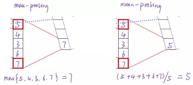
简单来说pooling操作可以进一步减少网络参数,通常max-pooling 对每一filter提取的向量进行操作,最后每一个filter对应一个数字。除此之外还有mean-pooling,就是将filter中的向量所有向量求平均得到一个数字。
这样操作过后4个5维的filter就转化成了1个4维的向量。而这个4维的向量就可以看成整段文本的的一个向量表示形式。得到了这个表示后,就可以将其应用在许多文本处理的问题中,比如简单的文本分类,聚类。
用DL4J实现基于CNN的文本分类
注意:
本示例需要额外引入deeplearning4j-nlp的Maven依赖
需要手动下载预训练的词向量和IMDB数据集,下载地址和存放路径在代码注释中。
运行时请将JVM的最大内存设置大一些,具体方法请查看注释。
import org.datavec.api.io.filters.BalancedPathFilter;
import org.datavec.api.io.labels.ParentPathLabelGenerator;
import org.datavec.api.split.FileSplit;
import org.datavec.api.split.InputSplit;
import org.datavec.image.loader.NativeImageLoader;
import org.datavec.image.recordreader.ImageRecordReader;
import org.datavec.image.transform.FlipImageTransform;
import org.datavec.image.transform.ImageTransform;
import org.datavec.image.transform.WarpImageTransform;
import org.deeplearning4j.datasets.datavec.RecordReaderDataSetIterator;
import org.deeplearning4j.datasets.iterator.MultipleEpochsIterator;
import org.deeplearning4j.eval.Evaluation;
import org.deeplearning4j.nn.api.OptimizationAlgorithm;
import org.deeplearning4j.nn.conf.*;
import org.deeplearning4j.nn.conf.inputs.InputType;
import org.deeplearning4j.nn.conf.layers.*;
import org.deeplearning4j.nn.multilayer.MultiLayerNetwork;
import org.deeplearning4j.nn.weights.WeightInit;
import org.deeplearning4j.optimize.listeners.ScoreIterationListener;
import org.deeplearning4j.util.ModelSerializer;
import org.nd4j.linalg.activations.Activation;
import org.nd4j.linalg.dataset.DataSet;
import org.nd4j.linalg.dataset.api.iterator.DataSetIterator;
import org.nd4j.linalg.dataset.api.preprocessor.DataNormalization;
import org.nd4j.linalg.dataset.api.preprocessor.ImagePreProcessingScaler;
import org.nd4j.linalg.learning.config.Nesterovs;
import org.nd4j.linalg.lossfunctions.LossFunctions;
import org.slf4j.Logger;
import org.slf4j.LoggerFactory;

import java.io.File;
import java.util.Arrays;
import java.util.List;
import java.util.Random;


/**
 * 用LeNet(一种卷积神经网络)对4类动物的图像进行分类
 * 该示例用较为简单的卷积网络模型LeNet和较低的分辨率(60*60*3),训练得到的模型准确率较低
 * 可以尝试讲模型修改为较为复杂的网络模型和使用更高的分辨率以获得更高的准确率
 */

public class AnimalsClassification {
    protected static final Logger log = LoggerFactory.getLogger(AnimalsClassification.class);
    protected static int height = 60;
    protected static int width = 60;
    protected static int channels = 3;
    protected static int numExamples = 80;
    protected static int numLabels = 4;
    protected static int batchSize = 20;

    protected static long seed = 42;
    protected static Random rng = new Random(seed);

    protected static int iterations = 1;
    protected static int epochs = 200;
    protected static double splitTrainTest = 0.8;
    protected static boolean save = false;


    public void run(String[] args) throws Exception {

        log.info("Load data....");
        /**cd
         *
         * 下面的代码从文件夹中读取图片作为输入数据
         * 将每种类别的图片分别放在不同的文件夹下,并将这些文件夹放在同一个根目录下
         * DL4J会为不同文件夹下的图片分配不同个label,为相同文件夹下的图片分配相同的label
         **/
        ParentPathLabelGenerator labelMaker = new ParentPathLabelGenerator();
        File mainPath = new File("animals");
        FileSplit fileSplit = new FileSplit(mainPath, NativeImageLoader.ALLOWED_FORMATS, rng);
        BalancedPathFilter pathFilter = new BalancedPathFilter(rng, labelMaker, numExamples, numLabels, batchSize);

        //将数据分为训练数据和测试数据
        InputSplit[] inputSplit = fileSplit.sample(pathFilter, splitTrainTest, 1 - splitTrainTest);
        InputSplit trainData = inputSplit[0];
        InputSplit testData = inputSplit[1];

        //利用一些图像变换来生成一些训练数据
        ImageTransform flipTransform1 = new FlipImageTransform(rng);
        ImageTransform flipTransform2 = new FlipImageTransform(new Random(123));
        ImageTransform warpTransform = new WarpImageTransform(rng, 42);
        List<ImageTransform> transforms = Arrays.asList(new ImageTransform[]{flipTransform1, warpTransform, flipTransform2});


        //归一化
        DataNormalization scaler = new ImagePreProcessingScaler(0, 1);

        log.info("Build model....");

        MultiLayerNetwork network = lenetModel();
        network.init();
        network.setListeners(new ScoreIterationListener(10));

        ImageRecordReader recordReader = new ImageRecordReader(height, width, channels, labelMaker);
        DataSetIterator dataIter;
        MultipleEpochsIterator trainIter;


        log.info("Train model....");
        // 用原始图像来训练
        recordReader.initialize(trainData, null);
        dataIter = new RecordReaderDataSetIterator(recordReader, batchSize, 1, numLabels);
        scaler.fit(dataIter);
        dataIter.setPreProcessor(scaler);
        trainIter = new MultipleEpochsIterator(epochs, dataIter);
        network.fit(trainIter);

        // 用变换的图像来训练
        for (ImageTransform transform : transforms) {
            System.out.print("\nTraining on transformation: " + transform.getClass().toString() + "\n\n");
            recordReader.initialize(trainData, transform);
            dataIter = new RecordReaderDataSetIterator(recordReader, batchSize, 1, numLabels);
            scaler.fit(dataIter);
            dataIter.setPreProcessor(scaler);
            trainIter = new MultipleEpochsIterator(epochs, dataIter);
            network.fit(trainIter);
        }


        //评价模型
        log.info("Evaluate model....");
        recordReader.initialize(testData);
        dataIter = new RecordReaderDataSetIterator(recordReader, batchSize, 1, numLabels);
        scaler.fit(dataIter);
        dataIter.setPreProcessor(scaler);
        Evaluation eval = network.evaluate(dataIter);
        log.info(eval.stats(true));

        // 取出第一条数据进行预测
        dataIter.reset();
        DataSet testDataSet = dataIter.next();
        List<String> allClassLabels = recordReader.getLabels();
        int labelIndex = testDataSet.getLabels().argMax(1).getInt(0);
        int[] predictedClasses = network.predict(testDataSet.getFeatures());
        String expectedResult = allClassLabels.get(labelIndex);
        String modelPrediction = allClassLabels.get(predictedClasses[0]);
        System.out.print("\nFor a single example that is labeled " + expectedResult + " the model predicted " + modelPrediction + "\n\n");

        // 保存模型
        if (save) {
            log.info("Save model....");
            ModelSerializer.writeModel(network, "model.bin", true);
        }
        log.info("****************Example finished********************");
    }

    private ConvolutionLayer convInit(String name, int in, int out, int[] kernel, int[] stride, int[] pad, double bias) {
        return new ConvolutionLayer.Builder(kernel, stride, pad).name(name).nIn(in).nOut(out).biasInit(bias).build();
    }

    private ConvolutionLayer conv5x5(String name, int out, int[] stride, int[] pad, double bias) {
        return new ConvolutionLayer.Builder(new int[]{5, 5}, stride, pad).name(name).nOut(out).biasInit(bias).build();
    }

    private SubsamplingLayer maxPool(String name, int[] kernel) {
        return new SubsamplingLayer.Builder(kernel, new int[]{2, 2}).name(name).build();
    }

    //构建LeNet
    public MultiLayerNetwork lenetModel() {
        MultiLayerConfiguration conf = new NeuralNetConfiguration.Builder()
                .seed(seed)
                .iterations(iterations)
                .regularization(false)
                .activation(Activation.RELU) // 用RELU激活
                .learningRate(1e-2) // 学习速率
                .weightInit(WeightInit.XAVIER)
                .optimizationAlgo(OptimizationAlgorithm.STOCHASTIC_GRADIENT_DESCENT)
                .updater(new Nesterovs(0.9))
                .list()
                .layer(0, convInit("cnn1", channels, 50, new int[]{5, 5}, new int[]{1, 1}, new int[]{0, 0}, 0))
                .layer(1, maxPool("maxpool1", new int[]{2, 2}))
                .layer(2, conv5x5("cnn2", 100, new int[]{5, 5}, new int[]{1, 1}, 0))
                .layer(3, maxPool("maxool2", new int[]{2, 2}))
                .layer(4, new DenseLayer.Builder().nOut(500).build())
                .layer(5, new OutputLayer.Builder(LossFunctions.LossFunction.NEGATIVELOGLIKELIHOOD)
                        .nOut(numLabels)
                        .activation(Activation.SOFTMAX)
                        .build())
                .backprop(true).pretrain(false)
                .setInputType(InputType.convolutional(height, width, channels))
                .build();

        return new MultiLayerNetwork(conf);

    }

    public static void main(String[] args) throws Exception {
        new AnimalsClassification().run(args);
    }

}
运行结果:
2017-10-14 14:43:36 INFO  Nd4jBackend:194 - Loaded [JCublasBackend] backend

2017-10-14 14:43:37 INFO  Reflections:229 - Reflections took 170 ms to scan
122 urls, producing 54501 keys and 58577 values

2017-10-14 14:43:37 INFO  NativeOpsHolder:49 - Number of threads used for
NativeOps: 32

2017-10-14 14:43:38 INFO  Reflections:229 - Reflections took 69 ms to scan
10 urls, producing 31 keys and 227 values

2017-10-14 14:43:38 INFO  DefaultOpExecutioner:565 - Backend used: [CUDA];
OS: [Windows 10]

2017-10-14 14:43:38 INFO  DefaultOpExecutioner:566 - Cores: [8]; Memory:
[6.9GB];

2017-10-14 14:43:38 INFO  DefaultOpExecutioner:567 - Blas vendor: [CUBLAS]

2017-10-14 14:43:38 INFO  CudaExecutioner:2116 - Device name: [GeForce GTX
1060 6GB]; CC: [6.1]; Total/free memory: [6442450944]

2017-10-14 14:43:39 INFO  Reflections:229 - Reflections took 992 ms to scan
99 urls, producing 2323 keys and 9555 values

2017-10-14 14:43:39 INFO  ComputationGraph:56 - Starting ComputationGraph
with WorkspaceModes set to [training: SINGLE; inference: SINGLE]

2017-10-14 14:43:40 INFO  Reflections:229 - Reflections took 100 ms to scan
10 urls, producing 407 keys and 1602 values

Number of parameters by layer:

   cnn3    90100

   cnn4    120100

   cnn5    150100

   globalPool  0

   out 602

Loading word vectors and creating DataSetIterators

Starting training

2017-10-14 14:45:18 INFO  Nd4jBlas:37 - Number of threads used for BLAS: 0

2017-10-14 14:45:20 INFO  ScoreIterationListener:64 - Score at iteration 0
is 0.7202949854867678

2017-10-14 14:47:15 INFO  ScoreIterationListener:64 - Score at iteration 100
is 0.6463996689421923

2017-10-14 14:48:35 INFO  ScoreIterationListener:64 - Score at iteration 200
is 0.4634944634627448

2017-10-14 14:49:42 INFO  ScoreIterationListener:64 - Score at iteration 300
is 0.401260720151129

2017-10-14 14:50:51 INFO  ScoreIterationListener:64 - Score at iteration 400
is 0.34404899690885465

2017-10-14 14:51:46 INFO  ScoreIterationListener:64 - Score at iteration 500
is 0.3989343702531156

2017-10-14 14:52:38 INFO  ScoreIterationListener:64 - Score at iteration 600
is 0.3147465993881237

2017-10-14 14:53:28 INFO  ScoreIterationListener:64 - Score at iteration 700
is 0.29517011246749025

Epoch 0 complete. Starting evaluation:

Examples labeled as Negative classified by model as Negative: 11371 times

Examples labeled as Negative classified by model as Positive: 1129 times

Examples labeled as Positive classified by model as Negative: 2948 times

Examples labeled as Positive classified by model as Positive: 9553 times

==========================Scores========================================

\# of classes:    2

Accuracy:        0.8369

Precision:       0.8442

Recall:          0.8369

F1 Score:        0.8241

========================================================================

Predictions for first negative review:

P(Negative) = 0.6227536797523499

P(Positive) = 0.37724635004997253
请继续关注“DeepLearning4j”教程。完整系列搜索查看,请PC登录http://www.zhuanzhi.ai, 搜索“DeepLearning4j”即可得。
对DeepLearning4j教程感兴趣的同学,欢迎进入我们的专知DeepLearning4j主题群一起交流、学习、讨论,扫一扫如下群二维码即可进入(先加微信小助手weixinhao: Rancho_Fang,注明Deeplearning4j)。

展开全文
