实战 | Pytorch BiLSTM + CRF做NER

作者:我近视
https://zhuanlan.zhihu.com/p/59845590
说明: 本篇文章为Pytorch官网上BiLSTM CRF的说明
一. BILSTM + CRF介绍
jianshu.com/p/97cb3b6db
1.介绍
基于神经网络的方法,在命名实体识别任务中非常流行和普遍。如果你不知道Bi-LSTM和CRF是什么,你只需要记住他们分别是命名实体识别模型中的两个层。
1.1开始之前
我们假设我们的数据集中有两类实体——人名和地名,与之相对应在我们的训练数据集中,有五类标签:
B-Person, I- Person,B-Organization,I-Organization
假设句子x由五个字符w1,w2,w3,w4,w5组成,其中【w1,w2】为人名类实体,【w3】为地名类实体,其他字符标签为“O”。
1.2BiLSTM-CRF模型
以下将给出模型的结构:
第一,句子x中的每一个单元都代表着由字嵌入或词嵌入构成的向量。其中,字嵌入是随机初始化的,词嵌入是通过数据训练得到的。所有的嵌入在训练过程中都会调整到最优。
第二,这些字或词嵌入为BiLSTM-CRF模型的输入,输出的是句子x中每个单元的标签。
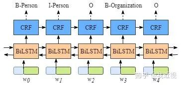
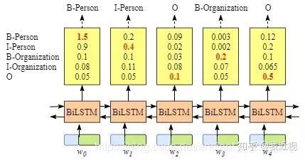
尽管一般不需要详细了解BiLSTM层的原理,但是为了更容易知道CRF层的运行原理,我们需要知道BiLSTM的输出层。
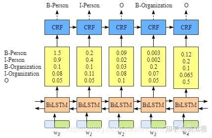
如上图所示,BiLSTM层的输出为每一个标签的预测分值,例如,对于单元w0,BiLSTM层输出的是
1.5 (B-Person), 0.9 (I-Person), 0.1 (B-Organization), 0.08 (I-Organization) 0.05 (O).
这些分值将作为CRF的输入。### 1.3 如果没有CRF层会怎样
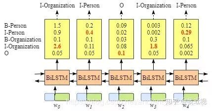
你也许已经发现了,即使没有CRF层,我们也可以训练一个BiLSTM命名实体识别模型,如图所示:
由于BiLSTM的输出为单元的每一个标签分值,我们可以挑选分值最高的一个作为该单元的标签。例如,对于单元w0,“B-Person”有最高分值—— 1.5,因此我们可以挑选“B-Person”作为w0的预测标签。同理,我们可以得到w1——“I-Person”,w2—— “O” ,w3——“B-Organization”,w4——“O”。
虽然我们可以得到句子x中每个单元的正确标签,但是我们不能保证标签每次都是预测正确的。例如,图4.中的例子,标签序列是“I-Organization I-Person” and “B-Organization I-Person”,很显然这是错误的。
1.4 CRF层能从训练数据中获得约束性的规则
CRF层可以为最后预测的标签添加一些约束来保证预测的标签是合法的。在训练数据训练过程中,这些约束可以通过CRF层自动学习到。 这些约束可以是: I:句子中第一个词总是以标签“B-“ 或 “O”开始,而不是“I-” II:标签“B-label1 I-label2 I-label3 I-…”,label1, label2, label3应该属于同一类实体。
例如,“B-Person I-Person” 是合法的序列, 但是“B-Person I-Organization” 是非法标签序列. III:标签序列“O I-label” is 非法的.实体标签的首个标签应该是 “B-“ ,而非 “I-“, 换句话说,有效的标签序列应该是“O B-label”。 有了这些约束,标签序列预测中非法序列出现的概率将会大大降低。
二. 标签的score和损失函数的定义
zhuanlan.zhihu.com/p/27
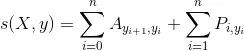
Bi-LSTM layer的输出维度是tag size,这就相当于是每个词 w~i~ 映射到tag的发射概率值,设Bi-LSTM的输出矩阵为P,其中P~i,j~代表词w~i~映射到tag~j~的非归一化概率。
对于CRF来说,我们假定存在一个转移矩阵A,则A~i,j~代表tag~i~转移到tag~j~的转移概率。 对于输入序列 X 对应的输出tag序列 y,定义分数为
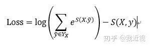
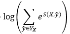
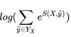
利用Softmax函数,我们为每一个正确的tag序列y定义一个概率值(Y~X~代表所有的tag序列,包括不可能出现的)

因而在训练中,我们只需要最大化似然概率p(y|X)即可,这里我们利用对数似然

所以我们将损失函数定义为-log(p(y|X)),就可以利用梯度下降法来进行网络的学习了。 loss function:
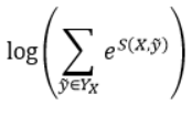
在对损失函数进行计算的时候,S(X,y)的计算很简单,而
(下面记作logsumexp)的计算稍微复杂一些,因为需要计算每一条可能路径的分数。这里用一种简便的方法,对于到词w~i+1~的路径,可以先把到词w~i~的logsumexp计算出来,因为

因此先计算每一步的路径分数和直接计算全局分数相同,但这样可以大大减少计算的时间。
三. 对于损失函数的详细解释
这篇文章对于理解十分有用
blog.csdn.net/cuihuijun
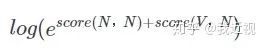
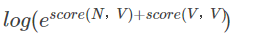
举例说 【我 爱 中国人民】对应标签【N V N】那这个标签就是一个完整的路径,也就对应一个Score值。 接下来我想讲的是这个公式:
这个公式成立是很显然的,动笔算一算就知道了,代码里其实就是用了这个公式的原理。
def _forward_alg(self, feats):
        # Do the forward algorithm to compute the partition function
        init_alphas = torch.full((1, self.tagset_size), -10000.)
        # START_TAG has all of the score.
        init_alphas[0][self.tag_to_ix[START_TAG]] = 0.

        # Wrap in a variable so that we will get automatic backprop
        forward_var = init_alphas

        # Iterate through the sentence
        for feat in feats:
            alphas_t = []  # The forward tensors at this timestep
            for next_tag in range(self.tagset_size):
                # broadcast the emission score: it is the same regardless of
                # the previous tag
                emit_score = feat[next_tag].view(
                    1, -1).expand(1, self.tagset_size)
                # the ith entry of trans_score is the score of transitioning to
                # next_tag from i
                trans_score = self.transitions[next_tag].view(1, -1)
                # The ith entry of next_tag_var is the value for the
                # edge (i -> next_tag) before we do log-sum-exp
                next_tag_var = forward_var + trans_score + emit_score
                # The forward variable for this tag is log-sum-exp of all the
                # scores.
                alphas_t.append(log_sum_exp(next_tag_var).view(1))
            forward_var = torch.cat(alphas_t).view(1, -1)
        terminal_var = forward_var + self.transitions[self.tag_to_ix[STOP_TAG]]
        alpha = log_sum_exp(terminal_var)
        return alpha
我们看到有这么一段代码 :
next_tag_var = forward_var + trans_score + emit_score我们主要就是来讲讲他。 首先这个算法的思想是:假设我们要做一个词性标注的任务,对句子【我 爱 中华人民】,我们要对这个句子做
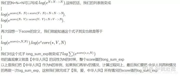
意思就是 对这个句子所有可能的标注,都算出来他们的Score,然后按照指数次幂加起来,再取对数。一般来说取所有可能的标注情况比较复杂,我们这里举例是长度为三,但是实际过程中,可能比这个要大得多,所以我们需要有一个简单高效得算法。也就是我们程序中得用得算法, 他是这么算得: 先算出【我, 爱】可能标注得所有情况,取 log_sum_exp 然后加上 转换到【中国人民】得特征值 再加上【中国人民】对应得某个标签得特征值。其等价于【我,爱,中国人民】所有可能特征值指数次幂相加,然后取对数. 接下来我们来验证一下是不是这样
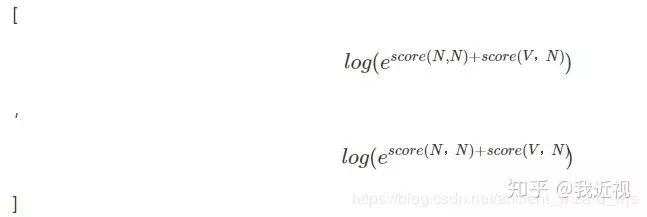
首先我们假设词性一共只有两种 名词N 和 动词 V 那么【我,爱】得词性组合一共有四种 N + N,N + V, V + N, V + V 那么【爱】标注为N时得log_sum_exp 为
【爱】 标注为 V时的 log_sum_exp为
我们的forward列表里就是存在着这两个值,即:
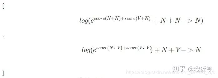
假设【中华人民】得词性为N,我们按照代码来写一下公式,在forward列表对应位置相加就是这样
四. 代码块详细说明:
blog.csdn.net/Jason__Li
先说明两个重要的矩阵:
feats: 发射矩阵(emit score)是sentence 在embedding后,再经过LSTM后得到的矩阵(也就是LSTM的输出), 维度为11 * 5 (11为sentence 的length,5是标签数)。 这个矩阵表示经过LSTM后sentence的每个word对应的每个labels的得分)。 表示发射概率。
self.transitions:转移矩阵,维度为55,transitions[i][j]表示label j转移到label i的概率。 transtion[i]维度为15,表示每个label转移到label i的概率。 表示概率矩阵
1. def log_sum_exp(vec)
# compute log sum exp in numerically stable way for the forward algorithm
def log_sum_exp(vec):   #vec是1*5, type是Variable
    max_score = vec[0, argmax(vec)]
    # max_score维度是1, max_score.view(1,-1)维度是1*1,
    # max_score.view(1, -1).expand(1, vec.size()[1])的维度是1*5
    max_score_broadcast = max_score.view(1, -1).expand(1, vec.size()[1])

    # 里面先做减法,减去最大值可以避免e的指数次,计算机上溢
    return max_score + \
        torch.log(torch.sum(torch.exp(vec - max_score_broadcast)))
你可能会疑问return 的结果为什么先减去max_score.其实这是一个小技巧,因为一上来就做指数运算可能会引起计算结果溢出,先减去score,经过log_sum_exp后,再把max_score给加上。 其实就等同于:
return torch.log(torch.sum(torch.exp(vec)))2. def neg_log_likelihood(self, sentence, tags)
如果你完整地把代码读完,你会发现neg_log_likelihood()这个函数是loss function.
loss = model.neg_log_likelihood(sentence_in, targets)我们来分析一下neg_log_likelihood()函数代码:
def neg_log_likelihood(self, sentence, tags):
        # feats: 11*5 经过了LSTM+Linear矩阵后的输出,之后作为CRF的输入。
        feats = self._get_lstm_features(sentence)
        forward_score = self._forward_alg(feats)
        gold_score = self._score_sentence(feats, tags)
return forward_score - gold_score你在这里可能会有疑问:问什么forward_score - gold_score可以作为loss呢。 这里,我们回顾一下我们在上文中说明的loss function函数公式:
你就会发现forward_score和gold_score分别表示上述等式右边的两项。
3. def _forward_alg(self, feats):
我们通过上一个函数的分析得知这个函数就是用来求forward_score的,也就是loss function等式右边的第一项:
# 预测序列的得分
    # 只是根据随机的transitions,前向传播算出的一个score
    #用到了动态规划的思想,但因为用的是随机的转移矩阵,算出的值很大score>20
    def _forward_alg(self, feats):
        # do the forward algorithm to compute the partition function
        init_alphas = torch.full((1, self.tagset_size), -10000.) # 1*5 而且全是-10000

        # START_TAG has all of the score
        # 因为start tag是4,所以tensor([[-10000., -10000., -10000., 0., -10000.]]),
        # 将start的值为零,表示开始进行网络的传播,
        init_alphas[0][self.tag_to_ix[START_TAG]] = 0

        # warp in a variable so that we will get automatic backprop
        forward_var = init_alphas # 初始状态的forward_var,随着step t变化

        # iterate through the sentence
        # 会迭代feats的行数次
        for feat in feats: #feat的维度是5 依次把每一行取出来~
            alphas_t = [] # the forward tensors at this timestep
            for next_tag in range(self.tagset_size): #next tag 就是简单 i,从0到len
                # broadcast the emission(发射) score:
                # it is the same regardless of the previous tag
                # 维度是1*5 LSTM生成的矩阵是emit score
                emit_score = feat[next_tag].view(
                    1, -1).expand(1, self.tagset_size)

                # the i_th entry of trans_score is the score of transitioning
                # to next_tag from i
                trans_score = self.transitions[next_tag].view(1, -1) # 维度是1*5

                # The ith entry of next_tag_var is the value for the
                # edge (i -> next_tag) before we do log-sum-exp
                # 第一次迭代时理解:
                # trans_score所有其他标签到B标签的概率
                # 由lstm运行进入隐层再到输出层得到标签B的概率,emit_score维度是1*5,5个值是相同的
                next_tag_var = forward_var + trans_score + emit_score

                # The forward variable for this tag is log-sum-exp of all the scores
                alphas_t.append(log_sum_exp(next_tag_var).view(1))
                # 此时的alphas t 是一个长度为5,例如<class 'list'>:
                # [tensor(0.8259), tensor(2.1739), tensor(1.3526), tensor(-9999.7168), tensor(-0.7102)]
            forward_var = torch.cat(alphas_t).view(1, -1) #到第(t-1)step时5个标签的各自分数
        # 最后只将最后一个单词的forward var与转移 stop tag的概率相加
        # tensor([[   21.1036,    18.8673,    20.7906, -9982.2734, -9980.3135]])
        terminal_var = forward_var + self.transitions[self.tag_to_ix[STOP_TAG]]
        alpha = log_sum_exp(terminal_var) # alpha是一个0维的tensor

        return alpha
4. def _score_sentence(self, feats, tags)
由2的函数分析,我们知道这个函数就是求gold_score,即loss function的第二项
# 根据真实的标签算出的一个score,
    # 这与上面的def _forward_alg(self, feats)共同之处在于:
    # 两者都是用的随机转移矩阵算的score
    # 不同地方在于,上面那个函数算了一个最大可能路径,但实际上可能不是真实的各个标签转移的值
    # 例如:真实标签是N V V,但是因为transitions是随机的,所以上面的函数得到其实是N N N这样,
    # 两者之间的score就有了差距。而后来的反向传播,就能够更新transitions,使得转移矩阵逼近
    #真实的“转移矩阵”

    # 得到gold_seq tag的score 即根据真实的label 来计算一个score,
    # 但是因为转移矩阵是随机生成的,故算出来的score不是最理想的值
    def _score_sentence(self, feats, tags): #feats 11*5  tag 11 维
        # gives the score of a provied tag sequence
        score = torch.zeros(1)

        # 将START_TAG的标签3拼接到tag序列最前面,这样tag就是12个了
        tags = torch.cat([torch.tensor([self.tag_to_ix[START_TAG]], dtype=torch.long), tags])

        for i, feat in enumerate(feats):
            # self.transitions[tags[i + 1], tags[i]] 实际得到的是从标签i到标签i+1的转移概率
            # feat[tags[i+1]], feat是step i 的输出结果,有5个值,
            # 对应B, I, E, START_TAG, END_TAG, 取对应标签的值
            # transition【j,i】 就是从i ->j 的转移概率值
            score = score + \
                self.transitions[tags[i+1], tags[i]] + feat[tags[i + 1]]
        score = score + self.transitions[self.tag_to_ix[STOP_TAG], tags[-1]]
        return score
5. def _viterbi_decode(self, feats):
# 维特比解码, 实际上就是在预测的时候使用了, 输出得分与路径值
    # 预测序列的得分
    def _viterbi_decode(self, feats):
        backpointers = []

        # initialize the viterbi variables in long space
        init_vvars = torch.full((1, self.tagset_size), -10000.)
        init_vvars[0][self.tag_to_ix[START_TAG]] = 0

        # forward_var at step i holds the viterbi variables for step i-1
        forward_var = init_vvars
        for feat in feats:
            bptrs_t = [] # holds the backpointers for this step
            viterbivars_t = [] # holds the viterbi variables for this step

            for next_tag in range(self.tagset_size):
                # next-tag_var[i] holds the viterbi variable for tag i
                # at the previous step, plus the score of transitioning
                # from tag i to next_tag.
                # we don't include the emission scores here because the max
                # does not depend on them(we add them in below)
                # 其他标签(B,I,E,Start,End)到标签next_tag的概率
                next_tag_var = forward_var + self.transitions[next_tag]
                best_tag_id = argmax(next_tag_var)
                bptrs_t.append(best_tag_id)
                viterbivars_t.append(next_tag_var[0][best_tag_id].view(1))
            # now add in the emssion scores, and assign forward_var to the set
            # of viterbi variables we just computed
            # 从step0到step(i-1)时5个序列中每个序列的最大score
            forward_var = (torch.cat(viterbivars_t) + feat).view(1, -1)
            backpointers.append(bptrs_t) # bptrs_t有5个元素

        # transition to STOP_TAG
        # 其他标签到STOP_TAG的转移概率
        terminal_var = forward_var + self.transitions[self.tag_to_ix[STOP_TAG]]
        best_tag_id = argmax(terminal_var)
        path_score = terminal_var[0][best_tag_id]

        # follow the back pointers to decode the best path
        best_path = [best_tag_id]
        for bptrs_t in reversed(backpointers):
            best_tag_id = bptrs_t[best_tag_id]
            best_path.append(best_tag_id)
        # pop off the start tag
        # we don't want to return that ti the caller
        start = best_path.pop()
        assert start == self.tag_to_ix[START_TAG] # Sanity check
        best_path.reverse() # 把从后向前的路径正过来
        return path_score, best_path
如果对于该函数还没有太理解,可以参考这篇博客:
blog.csdn.net/appleml/a
总结
以上就是我结合了几篇比较不错的博客后的总结,欢迎大家提问。


推荐阅读
征稿启示| 200元稿费+5000DBC(价值20个小时GPU算力)
完结撒花!李宏毅老师深度学习与人类语言处理课程视频及课件(附下载)
模型压缩实践系列之——bert-of-theseus,一个非常亲民的bert压缩方法
文本自动摘要任务的“不完全”心得总结番外篇——submodular函数优化
斯坦福大学NLP组Python深度学习自然语言处理工具Stanza试用
关于AINLP
AINLP 是一个有趣有AI的自然语言处理社区,专注于 AI、NLP、机器学习、深度学习、推荐算法等相关技术的分享,主题包括文本摘要、智能问答、聊天机器人、机器翻译、自动生成、知识图谱、预训练模型、推荐系统、计算广告、招聘信息、求职经验分享等,欢迎关注!加技术交流群请添加AINLPer(id:ainlper),备注工作/研究方向+加群目的。

阅读至此了,分享、点赞、在看三选一吧🙏