初探Video Transformer(一):抛弃CNN的纯Transformer视频理解框架—TimeSformer

极市导读
Transformers开始在视频识别领域的“猪突猛进”,各种改进和魔改层出不穷。由此作者将开启Video Transformer系列的讲解,本篇主要介绍了FBAI团队的TimeSformer,这也是第一篇使用纯Transformer结构在视频识别上的文章。 >>加入极市CV技术交流群,走在计算机视觉的最前沿
paper: https://arxiv.org/abs/2102.05095
code(offical): https://github.com/facebookresearch/TimeSformer
accept: ICML2021
author: Facebook AI
一、前言
Transformers(VIT)在图像识别领域大展拳脚,超越了很多基于Convolution的方法。视频识别领域的Transformers也开始'猪突猛进',各种改进和魔改也是层出不穷,本篇博客讲解一下FBAI团队的TimeSformer,这也是第一篇使用纯Transformer结构在视频识别上的文章。
二、出发点
Video vs Image
-
Video是具有时序信息的,多个帧来表达行为或者动作,相比于Image直接理解pixel的内容而言,Video需要理解temporal的信息。
Transformer vs CNNs
-
相比于Convolution,Transformer没有很强的归纳偏置,可以更好的适合大规模的数据集。 -
Convolution的kernel被用来设计获取局部特征的,所以不能对超出'感受野'的特征信息进行建模,无法更好的感知全局特征。而Transformer的 self-attention机制不仅可以获取局部特征同时本身就具备全局特征感知能力。 -
Transformer具备更快的训练和推理的速度, 可以在与CNNS在相同的计算下构建具有更大学习能力的模型。(这个来自于VIT) -
可以把video视作为来自于各个独立帧的patch集合的序列,所以可以直接适用于VIT结构。
Transfomrer自身问题
-
self-attention的计算复杂程度跟token的数量直接相关,对于video来说,相比于图像会有更多的token(有N帧), 计算量会更大。
三、算法设计
Transformers有这么多的优点,所以既要保留纯粹的Transformer结构,同时要修改self-attention使其计算量降低并且可以构建Temporal特征。
构建VideoTransformer
我们先梳理一下Video怎么输入到Transformer中: 对于Video来说,输入为 , 表示为F帧采样的尺寸为 的RGB图像。Transformer需要patch构建sequence进行输入,所以有 ,这里 表示的是patchsize大小, 表示的是每帧有多少个patch。展开后,可以表示为向量。
对输入做Embeeding处理,, 这里
表示为一个可学习的矩阵,
表示一个可学习空间位置编码。相比于Image的cls-token,Video的cls-token表示为
。
Transformer整体包含L层encoding blocks, 每个block的query,key,value表达如下:
这里, 表示attention heads数量, 表示的是每个head的维度。
相比于Image的self-attention, Video的self-attention需要计算temporal维度,公式表达为:
Note: 公式里把cls-token单独提出来了,这样方便表达空间和时序维度的attention。
合并每个heads的attention后,进行一个线性投影,送入MLP中,同时进行一个残差连接和Image的Transformer没有区别,公式表达如下:
最后就是分类层了,取cls-token用于最终的分类。
这样,我们就可以得到一个从输入到输出的VideoTransformer的完整表示。知道了怎么输入输出,接下来讨论怎么改进更好的获取temporal特征信息。
Self-Attention范式
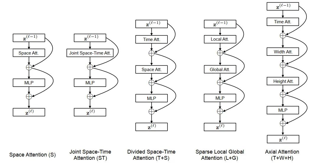
为了解决时序的问题,文中提出了几种构建范式,如下图所示:
-
SpaceAttention(S)这种就是标准的Transformer结构了,不计算Temporal的信息,只计算空间信息。公式可以表达为:
-
Joint Space-Time Attention(ST)这种就是把temporal和空间的token拉伸在一起,计算量会变得很大( -> )。公式表达为:
-
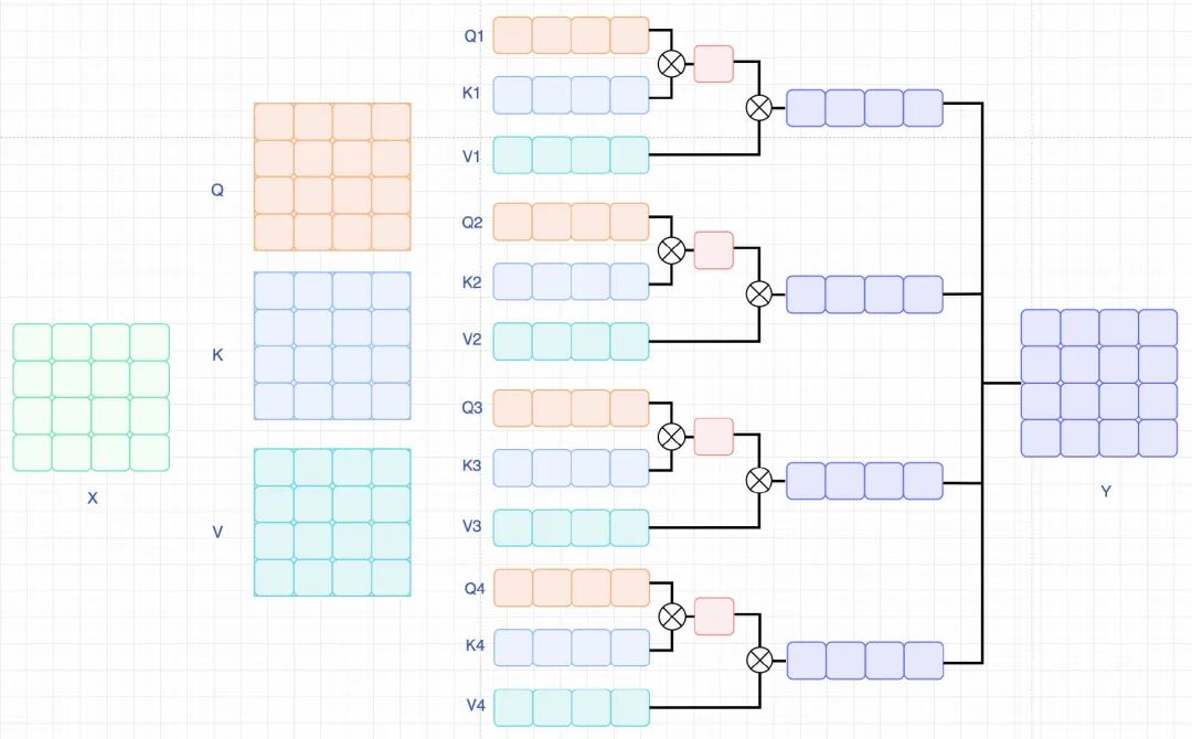
Divided Space-Time Attention(T+S)相比于前两种,这个变种的attention计算分成了两步,第一步计算Temporal-self-attention,第二步计算Spatial-self-attention,复杂度则会变为( -> ),每一次计算都会有
cls-token参与,所以需要+2。公式表达如下:两步独立计算且意义不同,所以Q,K,V需要来自不同的weights,不能共享权重。简单的定义为:
-
Sparse Local Global Attention (L+G)这个attention文章只做了简单的描述,没有给出相关代码实现,这里参考了Generating Long Sequences with Sparse Transformers(https://arxiv.org/pdf/1904.10509.pdf)文章,做一个简单的解释。
先引入几个概念和图示
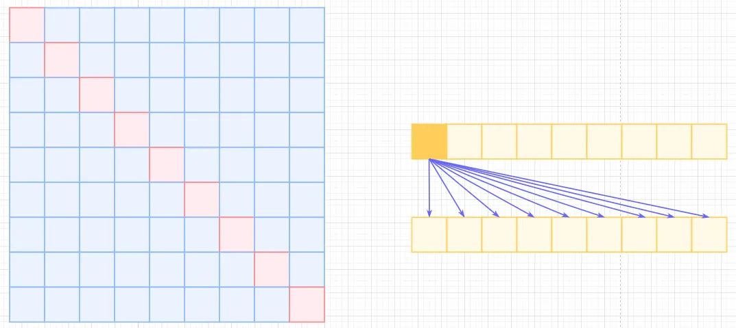
Self-Attention, 左边是self-attention矩阵,右边是对应的相乘关系,复杂度为 。
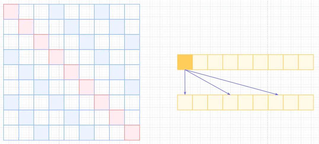
transformer Atrous Self-Attention,为了减少计算复杂度,引用空洞概念,类似于空洞卷积,只计算与之相关的k个元素计算,这样就会存在距离不满足k的倍数的注意力为0,相当于加了一个k的stride的滑窗,如下图中的白色位置。这样复杂度可以从 降低到 。
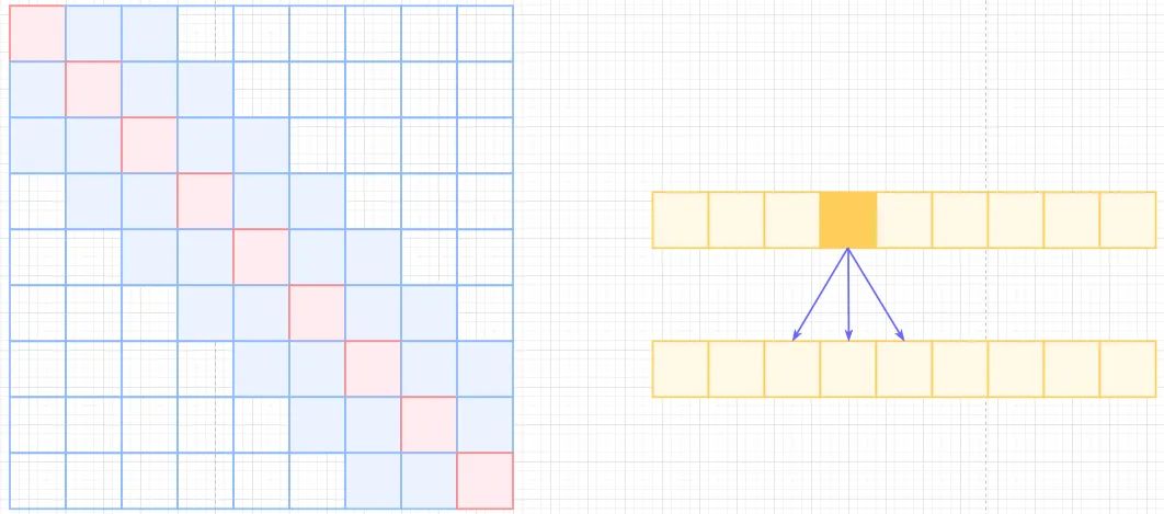
Atrous Self Attention Local Self-Attention, 标准self-attention是用来计算
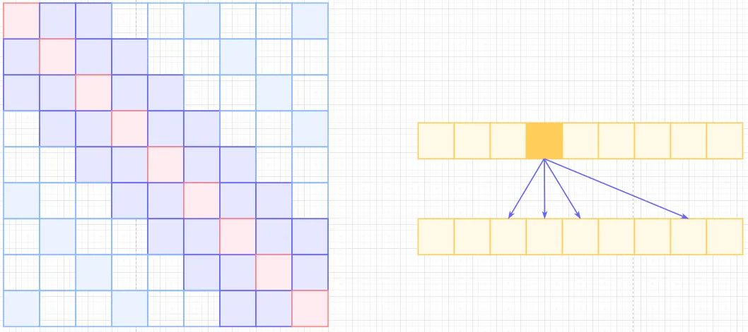
Non-Local的,那也可以引入局部关联来计算local的,很简单,约束每个元素与自己k个邻域元素有关即可,如下图,复杂度为 , 也就是 , 计算复杂度直接从平方降低到了线性,也损失了标准self-attention的长距离相关性。Local Self Attention Sparse Self-Attention, 所以有了OpenAI的Sparse self-attention,直接合并Local和Atrous,除了相对距离不超过k的,相对距离为k的倍数的注意力都为0,这样Attention就有了"局部紧密相关和远程稀疏相关"的特性。
Sparse Self Attention 回到本文,local-attention只考虑 的patches,也就是每个patch只关注1/4图像区域近邻的patchs,其他的patchs忽略。global-attention则采用2的stride来在Temporal维度和HW维度上进行patches的滑窗计算。与Sparser self-attention不同点在于,Sparse Local Global Attention先计算local后再进行计算global。
-
Axial Attention(T+W+H), 已经有很多的图像分类的paper讲过解耦attention,也就是用H或者W方向的attention单独计算,例如cswin-transformers里面的简单图示如下:
w self-attention 与之不同的是,Video不仅分行和列,还要分时序维度来进行计算,对应Q,K,V的weighis也各不相同。先计算Temporal-attention,然后Width-attention,最后Height-attention。行和列可以互换,不影响结果。
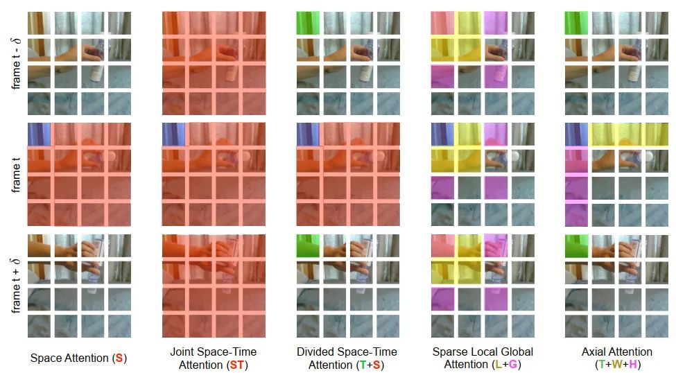
为了说明问题,用蓝色表示query patch,非蓝色的颜色表示在每种不同范式下与蓝色patch的自我注意力计算,不同颜色表示不同的维度来计算attention。
四、代码分析
论文中只给出了前三种attention的实现,所以我们就只分析前三种attention的code
PatchEmbed
Video的输入前面有介绍,是(B,C,T,H,W), 如果我们使用2d卷积的话,是没办法输入5个维度的,所以要合并F和B成一个维度,有(B,C,T,H,W)->((B,T),C,H,W)。和VIT一样,采用Conv2d做embeeding,代码如下,最终返回一个维度为((B,T), (H//P*W//P), D)的embeeding.
class PatchEmbed(nn.Module):
    """ Image to Patch Embedding
    """
    def __init__(self, img_size=224, patch_size=16, in_chans=3, embed_dim=768):
        super().__init__()
        img_size = to_2tuple(img_size)
        patch_size = to_2tuple(patch_size)
        num_patches = (img_size[1] // patch_size[1]) * (img_size[0] // patch_size[0])
        self.img_size = img_size
        self.patch_size = patch_size
        self.num_patches = num_patches

        self.proj = nn.Conv2d(in_chans, embed_dim, kernel_size=patch_size, stride=patch_size)

    def forward(self, x):
        B, C, T, H, W = x.shape
        x = rearrange(x, 'b c t h w -> (b t) c h w')
        x = self.proj(x)   # ((bt), dim, h//p, w//p)
        W = x.size(-1)
        x = x.flatten(2).transpose(1, 2)   # ((b, t), )
        return x, T, W                     # ((b, t), h//p * w//p, dims)
从patchEmbed得到的((B,T), nums_patches, dim),需要concat上一个clstoken用于最后的分类,所以有:
B = x.shape[0]
x, T, W = self.patch_embed(x)
cls_tokens = self.cls_token.expand(x.size(0), -1, -1)    #  ((bs, T), 1, dims)
x = torch.cat((cls_tokens, x), dim=1)                    #  ((bs, T), (nums+1), dims)
Space Attention
Space Attention已经介绍过了,只计算空间维度的atttention, 所以得到的embeeding直接送入到VIT的block里面。由于,T是合并到了BatchSize维度的,所以计算完attention后需要transpose回来,然后多帧取平均,最后送入MLP来做分类,代码如下:
## Attention blocks
def blocks(x):
    x = x + self.drop_path(self.attn(self.norm1(x)))
    x = x + self.drop_path(self.mlp(self.norm2(x)))
    return x

for blk in self.blocks:
    x = blk(x, B, T, W)

### Predictions for space-only baseline
if self.attention_type == 'space_only':
    x = rearrange(x, '(b t) n m -> b t n m',b=B,t=T)
    x = torch.mean(x, 1) # averaging predictions for every frame
Joint Space-Time Attention
Joint Space-Time Attention 需要引入TimeEmbeeding, 这个Embeeidng和PosEmbeeding类似,是可学习的,定义如下:
self.time_embed = nn.Parameter(torch.zeros(1, num_frames, embed_dim))
计算attention之前,需要引入TimeEmbeeding的信息到PatchEmbeeding,所以有:
cls_tokens = x[:B, 0, :].unsqueeze(1)               # (bs, 1, dims)
x = x[:,1:]                                         # ((bs, t), nums_patchs, dims)
x = rearrange(x, '(b t) n m -> (b n) t m',b=B,t=T)  # ((bs, nums_patches), t, dims)
x = x + self.time_embed                        # ((bs, nums_patches), t, dims)
# 为了加上timeembeeding
x = self.time_drop(x)
x = rearrange(x, '(b n) t m -> b (n t) m',b=B,t=T) # (bs, (nums_patches, t), dims)
x = torch.cat((cls_tokens, x), dim=1)              # (bs, (nums_patches, t)  + 1, dims)
由于已经合并了time和space的token计算,所以直接取cls-token进行分类即可。
## Attention blocks
for blk in self.blocks:
    x = blk(x, B, T, W)
Divided Space-Time Attention
Divided Space-Time Attention相对复杂一些,涉及比较多的shape转换。和Joint一样,也需要引入TimeEmbeeding,和上面一致,这里就不重复了。先把维度transpose为((B, nums_patches), T, Dims)进行时序的attention计算,并加上残差, 有:
## Temporal
xt = x[:,1:,:]                                                          # (bs, (nums_pathces, T), dims)
xt = rearrange(xt, 'b (h w t) m -> (b h w) t m',b=B,h=H,w=W,t=T)        # ((bs,  nums_pathces), T, dims)
res_temporal = self.drop_path(self.temporal_attn(self.temporal_norm1(xt)))  # ((bs,  nums_pathces), T, dims)
# 渐进式学习时间特征
res_temporal = self.temporal_fc(res_temporal)                                         # (bs, (nums_patches, T), dims)
xt = x[:,1:,:] + res_temporal                                                         # (bs, (nums_patches, T), dims)
这里有个特殊的层temporal_fc,文章中并没有提到过,但是作者在github的issue有回答,temporal_fc层首先以零权重初始化,因此在最初的训练迭代中,模型只利用空间信息。随着训练的进行,该模型会逐渐学会纳入时间信息。实验表明,这是一种训练TimeSformer的有效方法。(Note: 训练trick,没有的话可能会掉点)
temporal_fc = nn.Linear(dim, dim)

nn.init.constant_(temporal_fc.weight, 0)
nn.init.constant_(temporal_fc.bias, 0)
然后计算空间attention,这里要注意的是需要repeat和transpose cls-token的shape,原始的cls-token只表达spatial的所有信息,现在需要把temporal的信息融合进来,代码如下:
## Spatial
init_cls_token = x[:,0,:].unsqueeze(1)                                                # (bs, 1, dims)
cls_token = init_cls_token.repeat(1, T, 1)                                            # (bs, T, dims)
cls_token = rearrange(cls_token, 'b t m -> (b t) m', b=B, t=T).unsqueeze(1)           # ((bs, T), 1, dims)
xs = xt
xs = rearrange(xs, 'b (h w t) m -> (b t) (h w) m',b=B,h=H,w=W,t=T)                    # ((bs, T), num_patches, dims)
xs = torch.cat((cls_token, xs), 1)                                                    # ((bs, T), (num_patches + 1), dims)
res_spatial = self.drop_path(self.attn(self.norm1(xs)))                               # ((bs, T), (num_patches + 1), dims)
cls-token这里有两个作用,一个是保留原始特征信息并参与空间特征计算,另一个是融合时序特征。
### Taking care of CLS token
cls_token = res_spatial[:,0,:]                                                        # ((bs,  T), dims)
cls_token = rearrange(cls_token, '(b t) m -> b t m',b=B,t=T)                          # (bs, T,  dims)
cls_token = torch.mean(cls_token,1,True) ## averaging for every frame                 # (bs, 1, dims)
res_spatial = res_spatial[:,1:,:]                                                     # ((bs, T),  num_patches, dims)
res_spatial = rearrange(res_spatial, '(b t) (h w) m -> b (h w t) m',b=B,h=H,w=W,t=T)  # (bs, (num_patches, T), dims)
res = res_spatial
x = xt
第一部分就是带有原始cls-token的时序残差特征,第二部分就是融合时序特征的空间cls-token和spatial-attention,两部分相加,最后送入MLP,完成整个attention的计算。
# res
x = torch.cat((init_cls_token, x), 1) + torch.cat((cls_token, res), 1)                # (bs, (num_patches, T), dims)
## Mlp
x = x + self.drop_path(self.mlp(self.norm2(x)))
五、实验结果
Analysis of Self-Attention Schemes
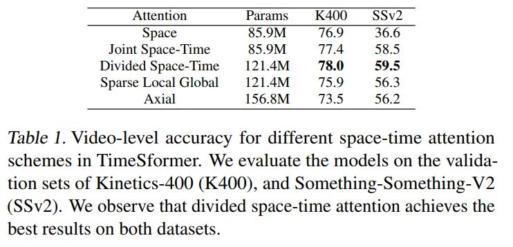
Attention实验结论很明显,K400和SSV2,Divided Space-Time效果是最好的, 比较有趣的是Space在K400的表现并不差,但是在SSV2上效果很差,说明SSV2数据集更加趋向于动作,K400更加趋向于内容。(NOTE: Joint Space-Time attention实际上使用了TimeEmbeeding的,实际参数量应该比Space多一点点,不过量级很少,所以这里没有标示。)
compare the computational cost
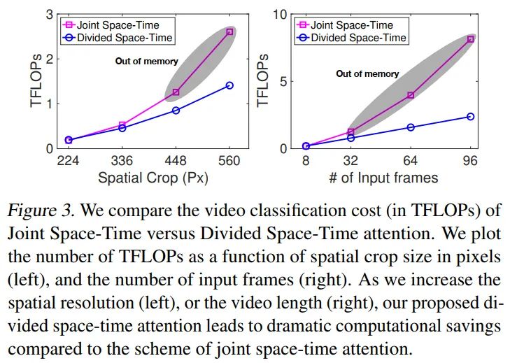
做了一下极限crop和frames的实验,可以看到Divided Space-time可以跑更大的分辨率且更多的帧,也就意味着可以刷更高的指标。
Comparison to 3D CNNs
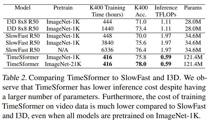
虽然TimeSformer的参数很大,但是推理开销更少,训练成本也更低,反之I3D,SlowFast这种3D CNNs需要更长的优化周期才能达到不错的性能。
The Importance of Pretraining
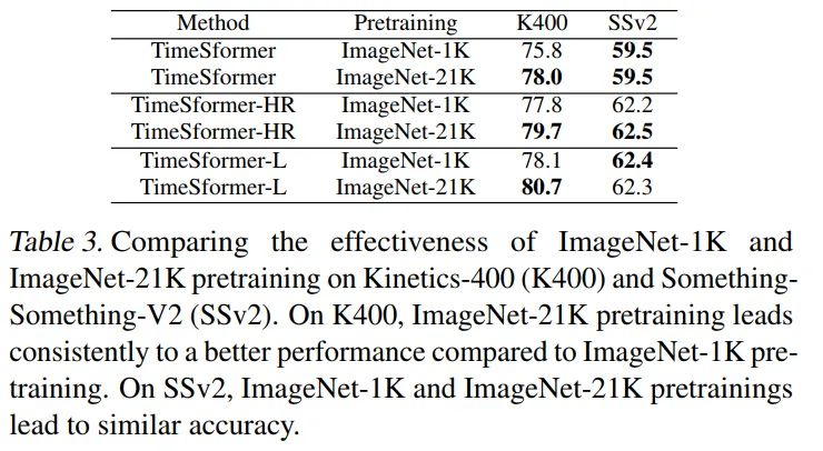
实验说明了一个问题,更NB的pretrain会带来更高的收益,TimeSformer表示的是8x224x224video片段输入,TimeSformer-HR表示的是16x448x448video片段输入,TimeSformer-L表示的是96x224x224video片段输入。
The Impact of Video-Data Scale
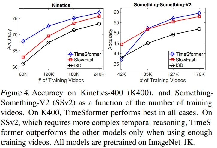
分开讨论,对于理解性的视频数据集,K400,TimeSfomer可以在少量数据集的情况下也超过I3D和SlowFast。对于时序性的数据,TimeSformer需要更多的数据集才能达到不错的效果。
The Importance of Positional Embeddings
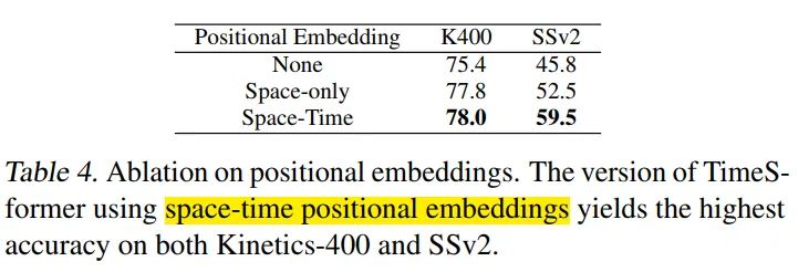
空间和时序的pos embeeding很重要,尤其是SSV2数据集上表现很明显。
Varying the Number of Tokens
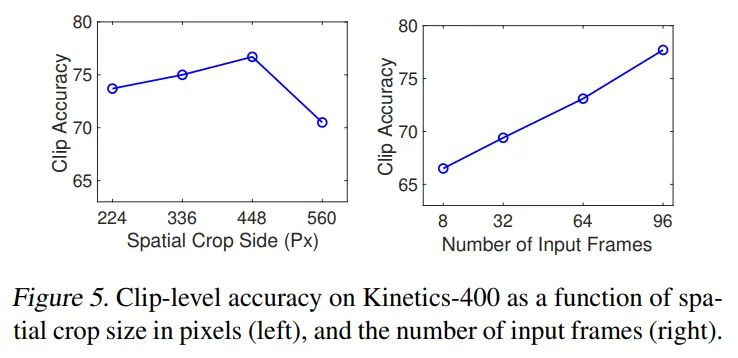
增加分辨率可以提升性能,增加视频采样帧数可以带来持续收益,最高可以达到96帧(GPU显存限制),已经远超cnn base的8-32帧。
Comparison to the State-of-the-Art
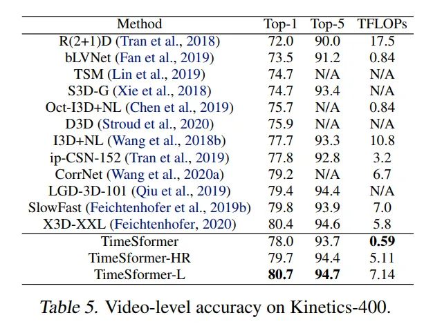
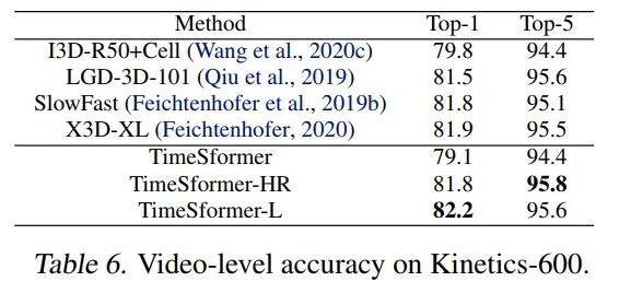
K400, TimeSformer采用的是3spatial crops(left,center,right)就可以达到80.7%的SOTA。K600,TimeSformer达到了82.2%的SOTA。
The effect of using multiple temporal clips
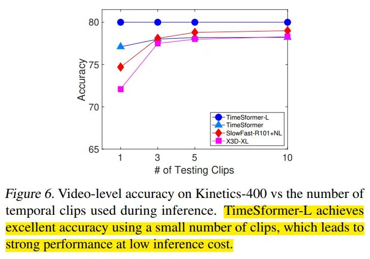
采用了{1,3,5,10}不同的clips数量,可以看到TimeSfomer-L的性能保持不变,TimeSfomer在3clips的时候性能保持稳定,X3D,SlowFast还会随着clips的增加(>=5)而提升性能。对于略短的视频片段来说,TimeSfomer可以用更少的推理开销达到很高的性能。
Something-Something-V2 & Diving-48
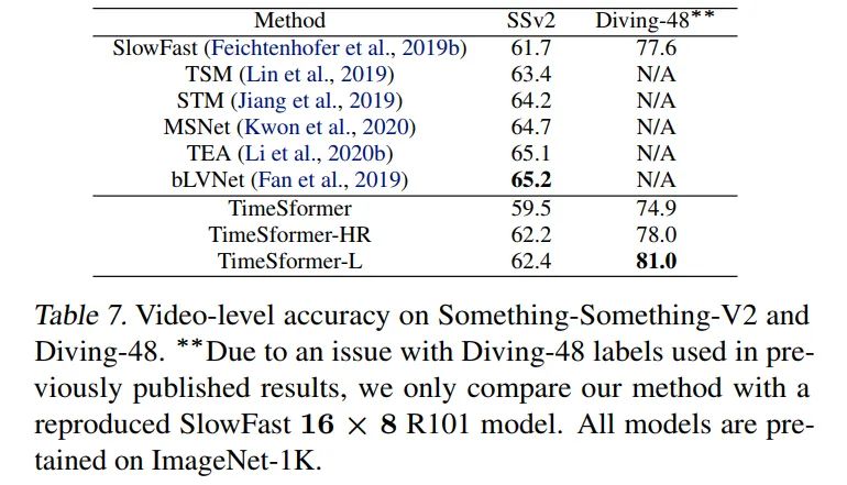
SSV2上的性能只比SlowFast高,甚至低于TSM,Diviing-48比SlowFast高了很多。
Long-Term Video Modeling
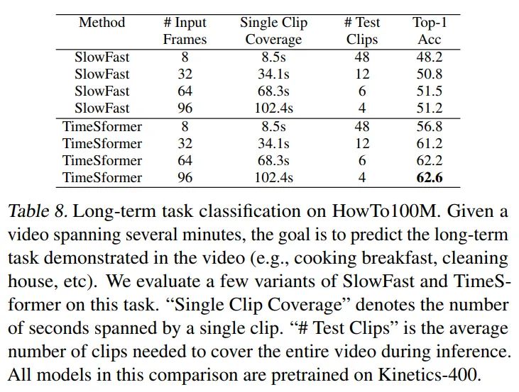
相比于SlowFast在长视频的表现,TimeSformer高出10个点左右,这个表里的数据是先用k400做pretrain后训练howto100得到的,使用imagenet21k做pretrain,最高可以达到62.1%,说明TimeSformer可以有效的训练长视频,不需要额外的pretrian数据。
Additional Ablations
-
Smaller&Larger Transformers Vit Large, k400和SSV2都降了1个点 相比vit base Vit Small, k400和SSV2都降了5个点 相比vit base
-
Larger Patch Size patchsize 从16调整为32,降低了3个点
-
The Order of Space and Time Self-Attention 调整空间attention在前,时序attention在后,降低了0.5个点 尝试了并行时序空间attention,降低了0.4个点
Visualizing Learned Space-Time Attention
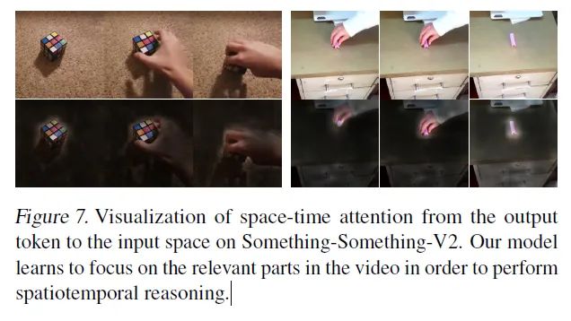
TimeSformer可以学会关注视频中的空间和时序相关部分,以便进行时空理解。
Visualizing Learned Feature Embeddings.
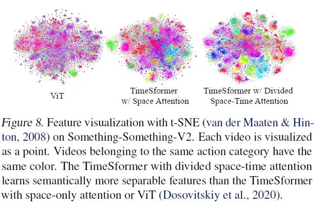
t-SNE显示,可以看到Divided Space-Time Attention的特征区分程度更强
六、结论
-
提出了基于Transformer的video模型范式,设计了divide sapce-time attention。 -
在K400,K600上取得了SOTA的效果。 -
相比于3D CNNs,训练和推理的成本低。 -
可以应用于超过一分钟的视频片段,具备长视频建模能力。
参考
如果觉得有用,就请分享到朋友圈吧!
公众号后台回复“transformer”获取最新Transformer综述论文下载~

# 极市平台签约作者#

FlyEgle
知乎:FlyEgle
欢聚时代算法工程师
领域:OCR, 图像视频内容理解,超分
github: https://github.com/FlyEgle