时间序列深度学习:状态 LSTM 模型预测太阳黑子(下)

2018 年 6 月 15 日 R语言中文社区

作者:徐瑞龙 整理分享量化投资与固定收益相关的文章

博客专栏: 

https://www.cnblogs.com/xuruilong100 


5.3 预测未来 10 年的数据

我们可以通过调整预测函数来使用完整的数据集预测未来 10 年的数据。新函数 predict_keras_lstm_future() 用来预测未来 120 步(或 10 年)的数据。

predict_keras_lstm_future <- function(data,
                                                            epochs = 300,                                      
                                                            ...) {        lstm_prediction <- function(data,                                                 epochs,                                
                                                ...) {                # 5.1.2 Data Setup (MODIFIED)        df <- data                # 5.1.3 Preprocessing        rec_obj <- recipe(value ~ ., df) %>%            
             step_sqrt(value) %>%            
             step_center(value) %>%            
             step_scale(value) %>%            
             prep()                df_processed_tbl <- bake(rec_obj, df)                center_history <- rec_obj$steps[[2]]$means["value"]        scale_history  <- rec_obj$steps[[3]]$sds["value"]                
       # 5.1.4 LSTM Plan        lag_setting  <- 120 # = nrow(df_tst)        batch_size   <- 40        train_length <- 440        tsteps       <- 1        epochs       <- epochs
                       # 5.1.5 Train Setup (MODIFIED)        lag_train_tbl <- df_processed_tbl %>%                                    mutate(                                        value_lag = lag(value, n = lag_setting)) %>%                                                    filter(!is.na(value_lag)) %>%                                                   tail(train_length)                x_train_vec <- lag_train_tbl$value_lag        x_train_arr <- array(                                    data = x_train_vec, dim = c(length(x_train_vec), 1, 1))                y_train_vec <- lag_train_tbl$value        y_train_arr <- array(                                    data = y_train_vec, dim = c(length(y_train_vec), 1))                x_test_vec <- y_train_vec %>% tail(lag_setting)        x_test_arr <- array(                                    data = x_test_vec, dim = c(length(x_test_vec), 1, 1))                        # 5.1.6 LSTM Model        model <- keras_model_sequential()        model %>%                                    layer_lstm(                                        units            = 50,                        input_shape      = c(tsteps, 1),                        batch_size       = batch_size,                                                        return_sequences = TRUE,                        stateful         = TRUE) %>%                                    layer_lstm(                                        units            = 50,                                         return_sequences = FALSE,                                                             stateful         = TRUE) %>%                        layer_dense(units = 1)                model %>%                                     compile(loss = 'mae', optimizer = 'adam')                # 5.1.7 Fitting LSTM        for (i in 1:epochs) {            model %>%                                       fit(x          = x_train_arr,                              y          = y_train_arr,                              batch_size = batch_size,                                                                  epochs     = 1,                              verbose    = 1,                              shuffle    = FALSE)                        model %>% reset_states()                                        cat("Epoch: ", i)                    }                # 5.1.8 Predict and Return Tidy Data (MODIFIED)        # Make Predictions        pred_out <- model %>%                                     predict(x_test_arr, batch_size = batch_size) %>%                                                 .[,1]                # Make future index using tk_make_future_timeseries()        idx <- data %>%                                    tk_index() %>%                                    tk_make_future_timeseries(n_future = lag_setting)                
                       # Retransform values        pred_tbl <- tibble(                                   index   = idx,                                                value   = (pred_out * scale_history + center_history)^2)              
                        # Combine actual data with predictions        tbl_1 <- df %>%                                     add_column(key = "actual")        tbl_3 <- pred_tbl %>%                                     add_column(key = "predict")        
                        # Create time_bind_rows() to solve dplyr issue        time_bind_rows <- function(data_1,                                                      data_2,                                                      index) {            index_expr <- enquo(index)                                     bind_rows(data_1, data_2) %>%                                             as_tbl_time(index = !! index_expr)        }        ret <- list(tbl_1, tbl_3) %>%                                     reduce(time_bind_rows, index = index) %>%                                                 arrange(key, index) %>%                                                 mutate(key = as_factor(key))                                             return(ret)            }        safe_lstm <- possibly(lstm_prediction, otherwise = NA)                                 safe_lstm(data, epochs, ...) }

下一步,在 sun_spots 数据集上运行 predict_keras_lstm_future() 函数。

future_sun_spots_tbl <- predict_keras_lstm_future(sun_spots, epochs = 300)

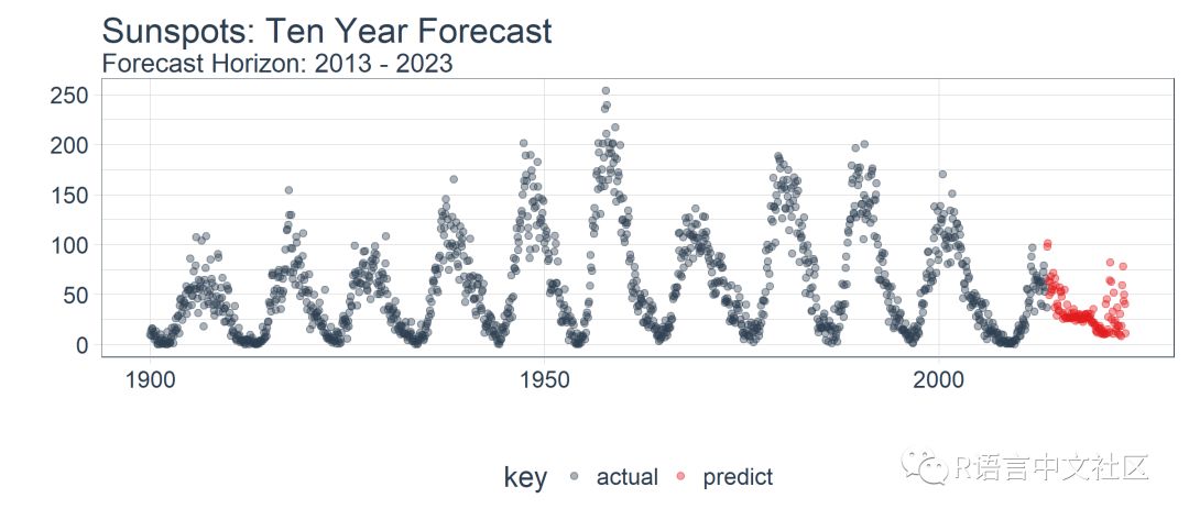
最后,我们使用 plot_prediction() 可视化预测结果,需要设置 id = NULL。我们使用 filter_time() 函数将数据集缩放到 1900 年之后。

future_sun_spots_tbl %>%

   filter_time("1900" ~ "end") %>%

   plot_prediction(

       id = NULL, alpha = 0.4, size = 1.5) +    

    theme(legend.position = "bottom") +    

    ggtitle(

       "Sunspots: Ten Year Forecast",

       subtitle = "Forecast Horizon: 2013 - 2023")

结论

本文演示了使用 keras 包构建的状态 LSTM 模型的强大功能。令人惊讶的是,提供的唯一特征是滞后 120 阶的历史数据,深度学习方法依然识别出了数据中的趋势。回测模型的 RMSE 均值等于 34,RMSE 标准差等于 13。虽然本文未显示,但我们对比测试1了 ARIMA 模型和 prophet 模型(Facebook 开发的时间序列预测模型),LSTM 模型的表现优越:平均误差减少了 30% 以上,标准差减少了 40%。这显示了机器学习工具-应用适合性的好处。

除了使用的深度学习方法之外,文章还揭示了使用 ACF 图确定 LSTM 模型对于给定时间序列是否适用的方法。我们还揭示了时间序列模型的准确性应如何通过回测来进行基准测试,这种策略保持了时间序列的连续性,可用于时间序列数据的交叉验证。


大家都在看

2017年R语言发展报告(国内)

R语言中文社区历史文章整理(作者篇)

R语言中文社区历史文章整理(类型篇)


公众号后台回复关键字即可学习

回复 R                  R语言快速入门及数据挖掘 
回复 Kaggle案例  Kaggle十大案例精讲(连载中)
回复 文本挖掘      手把手教你做文本挖掘
回复 可视化          R语言可视化在商务场景中的应用 
回复 大数据         大数据系列免费视频教程 
回复 量化投资      张丹教你如何用R语言量化投资 
回复 用户画像      京东大数据,揭秘用户画像
回复 数据挖掘     常用数据挖掘算法原理解释与应用
回复 机器学习     人工智能系列之机器学习与实践
回复 爬虫            R语言爬虫实战案例分享

登录查看更多
9

相关内容

长短期记忆网络(LSTM)是一种用于深度学习领域的人工回归神经网络(RNN)结构。与标准的前馈神经网络不同,LSTM具有反馈连接。它不仅可以处理单个数据点(如图像),还可以处理整个数据序列(如语音或视频)。例如,LSTM适用于未分段、连接的手写识别、语音识别、网络流量或IDSs(入侵检测系统)中的异常检测等任务。
Python数据分析:过去、现在和未来,52页ppt
专知会员服务
99+阅读 · 2020年3月9日
深度强化学习策略梯度教程,53页ppt
专知会员服务
175+阅读 · 2020年2月1日
【华侨大学】基于混合深度学习算法的疾病预测模型
专知会员服务
96+阅读 · 2020年1月21日
金融时序预测中的深度学习方法:2005到2019
专知会员服务
165+阅读 · 2019年12月4日
【电子书】让 PM 全面理解深度学习 65页PDF免费下载
专知会员服务
16+阅读 · 2019年10月30日
【新书】Python编程基础,669页pdf
专知会员服务
186+阅读 · 2019年10月10日
使用LSTM模型预测股价基于Keras
量化投资与机器学习
34+阅读 · 2018年11月17日
利用动态深度学习预测金融时间序列基于Python
量化投资与机器学习
18+阅读 · 2018年10月30日
基于 Keras 用 LSTM 网络做时间序列预测
R语言中文社区
21+阅读 · 2018年8月6日
基于 Keras 用深度学习预测时间序列
R语言中文社区
23+阅读 · 2018年7月27日
时间序列深度学习:状态 LSTM 模型预测太阳黑子(上)
R语言中文社区
19+阅读 · 2018年6月15日
教程 | 如何判断LSTM模型中的过拟合与欠拟合
机器之心
5+阅读 · 2017年10月2日
【推荐】一步一步带你用TensorFlow玩转LSTM
机器学习研究会
9+阅读 · 2017年9月12日
【推荐】用Tensorflow理解LSTM
机器学习研究会
36+阅读 · 2017年9月11日
【推荐】(Keras)LSTM多元时序预测教程
机器学习研究会
24+阅读 · 2017年8月14日
Do RNN and LSTM have Long Memory?
Arxiv
19+阅读 · 2020年6月10日
Learning Blind Video Temporal Consistency
Arxiv
3+阅读 · 2018年8月1日
Arxiv
5+阅读 · 2018年5月5日
Arxiv
5+阅读 · 2018年1月16日
Arxiv
5+阅读 · 2016年1月15日
Arxiv
4+阅读 · 2015年8月25日
VIP会员
相关资讯
使用LSTM模型预测股价基于Keras
量化投资与机器学习
34+阅读 · 2018年11月17日
利用动态深度学习预测金融时间序列基于Python
量化投资与机器学习
18+阅读 · 2018年10月30日
基于 Keras 用 LSTM 网络做时间序列预测
R语言中文社区
21+阅读 · 2018年8月6日
基于 Keras 用深度学习预测时间序列
R语言中文社区
23+阅读 · 2018年7月27日
时间序列深度学习:状态 LSTM 模型预测太阳黑子(上)
R语言中文社区
19+阅读 · 2018年6月15日
教程 | 如何判断LSTM模型中的过拟合与欠拟合
机器之心
5+阅读 · 2017年10月2日
【推荐】一步一步带你用TensorFlow玩转LSTM
机器学习研究会
9+阅读 · 2017年9月12日
【推荐】用Tensorflow理解LSTM
机器学习研究会
36+阅读 · 2017年9月11日
【推荐】(Keras)LSTM多元时序预测教程
机器学习研究会
24+阅读 · 2017年8月14日
相关论文
Do RNN and LSTM have Long Memory?
Arxiv
19+阅读 · 2020年6月10日
Learning Blind Video Temporal Consistency
Arxiv
3+阅读 · 2018年8月1日
Arxiv
5+阅读 · 2018年5月5日
Arxiv
5+阅读 · 2018年1月16日
Arxiv
5+阅读 · 2016年1月15日
Arxiv
4+阅读 · 2015年8月25日
Top
微信扫码咨询专知VIP会员