Keras集成梯度用于模型可解释性

【导读】集成梯度是一种用于将分类模型的预测归因于其输入特征的技术。这是一种模型可解释性技术：它来可视化输入要素和模型预测之间的关系。

原文链接：

https://keras.io/examples/vision/integrated_gradients/

介绍

集成梯度是在计算预测输出相对于输入特征的梯度时的变体。要计算集成梯度，我们需要执行以下步骤：

1. 识别输入和输出。在我们的例子中，输入是图像，输出是模型的最后一层（具有softmax激活的Dense层）。

2.在对特定数据点进行预测时，计算哪些特征对神经网络很重要。为了识别这些特征，我们需要选择一个基线输入。基线输入可以是黑色图像（所有像素值均设置为零）或随机噪声。基线输入的形状需要与我们的输入图像相同，例如（299，299，3）。

3. 在给定的步骤数内插基线。步数表示对于给定的输入图像，我们需要进行梯度近似的步骤。步骤数是一个超参数。作者建议使用20到1000步之间的任何步长。

4. 预处理这些插值图像并进行正向传递。

5. 获取这些插值图像的梯度。

6. 使用梯形法则近似梯度积分。

设置

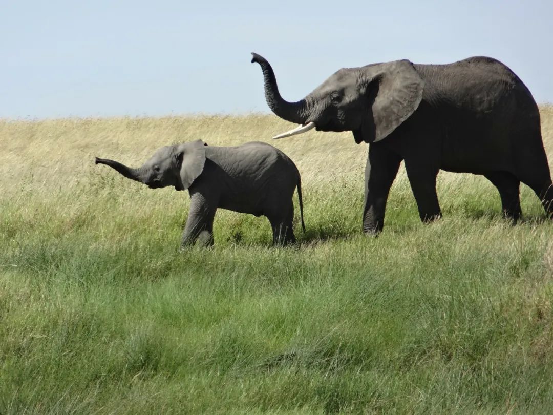
import numpy as npimport matplotlib.pyplot as pltfrom scipy import ndimagefrom IPython.display import Image
import tensorflow as tffrom tensorflow import kerasfrom tensorflow.keras import layersfrom tensorflow.keras.applications import xception
# Size of the input imageimg_size = (299, 299, 3)
# Load Xception model with imagenet weightsmodel = xception.Xception(weights="imagenet")
# The local path to our target imageimg_path = keras.utils.get_file("elephant.jpg", "https://i.imgur.com/Bvro0YD.png")display(Image(img_path))

显示图片

集成梯度算法

def get_img_array(img_path, size=(299, 299)):    # `img` is a PIL image of size 299x299img = keras.preprocessing.image.load_img(img_path, target_size=size)    # `array` is a float32 Numpy array of shape (299, 299, 3)array = keras.preprocessing.image.img_to_array(img)    # We add a dimension to transform our array into a "batch"    # of size (1, 299, 299, 3)array = np.expand_dims(array, axis=0)return array

def get_gradients(img_input, top_pred_idx):"""Computes the gradients of outputs w.r.t input image.
Args:img_input: 4D image tensortop_pred_idx: Predicted label for the input image
Returns:Gradients of the predictions w.r.t img_input"""images = tf.cast(img_input, tf.float32)
with tf.GradientTape() as tape:tape.watch(images)preds = model(images)top_class = preds[:, top_pred_idx]
grads = tape.gradient(top_class, images)return grads

def get_integrated_gradients(img_input, top_pred_idx, baseline=None, num_steps=50):"""Computes Integrated Gradients for a predicted label.
Args:img_input (ndarray): Original imagetop_pred_idx: Predicted label for the input imagebaseline (ndarray): The baseline image to start with for interpolationnum_steps: Number of interpolation steps between the baselineand the input used in the computation of integrated gradients. Thesesteps along determine the integral approximation error. By default,num_steps is set to 50.
Returns:Integrated gradients w.r.t input image"""    # If baseline is not provided, start with a black image    # having same size as the input image.if baseline is None:baseline = np.zeros(img_size).astype(np.float32)else:baseline = baseline.astype(np.float32)
    # 1. Do interpolation.img_input = img_input.astype(np.float32)interpolated_image = [baseline + (step / num_steps) * (img_input - baseline)for step in range(num_steps + 1)]interpolated_image = np.array(interpolated_image).astype(np.float32)
    # 2. Preprocess the interpolated imagesinterpolated_image = xception.preprocess_input(interpolated_image)
    # 3. Get the gradientsgrads = []for i, img in enumerate(interpolated_image):img = tf.expand_dims(img, axis=0)grad = get_gradients(img, top_pred_idx=top_pred_idx)grads.append(grad[0])grads = tf.convert_to_tensor(grads, dtype=tf.float32)
    # 4. Approximate the integral usiing the trapezoidal rulegrads = (grads[:-1] + grads[1:]) / 2.0avg_grads = tf.reduce_mean(grads, axis=0)
    # 5. Calculate integrated gradients and returnintegrated_grads = (img_input - baseline) * avg_gradsreturn integrated_grads

def random_baseline_integrated_gradients(img_input, top_pred_idx, num_steps=50, num_runs=2):"""Generates a number of random baseline images.
Args:img_input (ndarray): 3D imagetop_pred_idx: Predicted label for the input imagenum_steps: Number of interpolation steps between the baselineand the input used in the computation of integrated gradients. Thesesteps along determine the integral approximation error. By default,num_steps is set to 50.num_runs: number of baseline images to generate
Returns:Averaged integrated gradients for `num_runs` baseline images"""    # 1. List to keep track of Integrated Gradients (IG) for all the imagesintegrated_grads = []
    # 2. Get the integrated gradients for all the baselinesfor run in range(num_runs):baseline = np.random.random(img_size) * 255igrads = get_integrated_gradients(img_input=img_input,top_pred_idx=top_pred_idx,baseline=baseline,num_steps=num_steps,)integrated_grads.append(igrads)
    # 3. Return the average integrated gradients for the imageintegrated_grads = tf.convert_to_tensor(integrated_grads)return tf.reduce_mean(integrated_grads, axis=0)

可视化梯度与集成梯度

class GradVisualizer:"""Plot gradients of the outputs w.r.t an input image."""
def __init__(self, positive_channel=None, negative_channel=None):if positive_channel is None:self.positive_channel = [0, 255, 0]else:self.positive_channel = positive_channel
if negative_channel is None:self.negative_channel = [255, 0, 0]else:self.negative_channel = negative_channel
def apply_polarity(self, attributions, polarity):if polarity == "positive":return np.clip(attributions, 0, 1)else:return np.clip(attributions, -1, 0)
def apply_linear_transformation(self,attributions,clip_above_percentile=99.9,clip_below_percentile=70.0,lower_end=0.2,):        # 1. Get the thresholdsm = self.get_thresholded_attributions(attributions, percentage=100 - clip_above_percentile)e = self.get_thresholded_attributions(attributions, percentage=100 - clip_below_percentile)
        # 2. Transform the attributions by a linear function f(x) = a*x + b such that        # f(m) = 1.0 and f(e) = lower_endtransformed_attributions = (1 - lower_end) * (np.abs(attributions) - e) / (m - e) + lower_end
        # 3. Make sure that the sign of transformed attributions is the same as original attributionstransformed_attributions *= np.sign(attributions)
        # 4. Only keep values that are bigger than the lower_endtransformed_attributions *= transformed_attributions >= lower_end
        # 5. Clip values and returntransformed_attributions = np.clip(transformed_attributions, 0.0, 1.0)return transformed_attributions
def get_thresholded_attributions(self, attributions, percentage):if percentage == 100.0:return np.min(attributions)
        # 1. Flatten the attributionsflatten_attr = attributions.flatten()
        # 2. Get the sum of the attributionstotal = np.sum(flatten_attr)
        # 3. Sort the attributions from largest to smallest.sorted_attributions = np.sort(np.abs(flatten_attr))[::-1]
        # 4. Calculate the percentage of the total sum that each attribution        # and the values about it contribute.cum_sum = 100.0 * np.cumsum(sorted_attributions) / total
        # 5. Threshold the attributions by the percentageindices_to_consider = np.where(cum_sum >= percentage)[0][0]
        # 6. Select the desired attributions and returnattributions = sorted_attributions[indices_to_consider]return attributions
def binarize(self, attributions, threshold=0.001):return attributions > threshold
def morphological_cleanup_fn(self, attributions, structure=np.ones((4, 4))):closed = ndimage.grey_closing(attributions, structure=structure)opened = ndimage.grey_opening(closed, structure=structure)return opened
def draw_outlines(self, attributions, percentage=90, connected_component_structure=np.ones((3, 3))):        # 1. Binarize the attributions.attributions = self.binarize(attributions)
        # 2. Fill the gapsattributions = ndimage.binary_fill_holes(attributions)
        # 3. Compute connected componentsconnected_components, num_comp = ndimage.measurements.label(attributions, structure=connected_component_structure)
        # 4. Sum up the attributions for each componenttotal = np.sum(attributions[connected_components > 0])component_sums = []for comp in range(1, num_comp + 1):mask = connected_components == compcomponent_sum = np.sum(attributions[mask])component_sums.append((component_sum, mask))
        # 5. Compute the percentage of top components to keepsorted_sums_and_masks = sorted(component_sums, key=lambda x: x[0], reverse=True)sorted_sums = list(zip(*sorted_sums_and_masks))[0]cumulative_sorted_sums = np.cumsum(sorted_sums)cutoff_threshold = percentage * total / 100cutoff_idx = np.where(cumulative_sorted_sums >= cutoff_threshold)[0][0]if cutoff_idx > 2:cutoff_idx = 2
        # 6. Set the values for the kept componentsborder_mask = np.zeros_like(attributions)for i in range(cutoff_idx + 1):border_mask[sorted_sums_and_masks[i][1]] = 1
        # 7. Make the mask hollow and show only the bordereroded_mask = ndimage.binary_erosion(border_mask, iterations=1)border_mask[eroded_mask] = 0
        # 8. Return the outlined maskreturn border_mask
def process_grads(self,image,attributions,polarity="positive",clip_above_percentile=99.9,clip_below_percentile=0,morphological_cleanup=False,structure=np.ones((3, 3)),outlines=False,outlines_component_percentage=90,overlay=True,):if polarity not in ["positive", "negative"]:raise ValueError(f""" Allowed polarity values: 'positive' or 'negative'but provided {polarity}""")if clip_above_percentile < 0 or clip_above_percentile > 100:raise ValueError("clip_above_percentile must be in [0, 100]")
if clip_below_percentile < 0 or clip_below_percentile > 100:raise ValueError("clip_below_percentile must be in [0, 100]")
        # 1. Apply polarityif polarity == "positive":attributions = self.apply_polarity(attributions, polarity=polarity)channel = self.positive_channelelse:attributions = self.apply_polarity(attributions, polarity=polarity)attributions = np.abs(attributions)channel = self.negative_channel
        # 2. Take average over the channelsattributions = np.average(attributions, axis=2)
        # 3. Apply linear transformation to the attributionsattributions = self.apply_linear_transformation(attributions,clip_above_percentile=clip_above_percentile,clip_below_percentile=clip_below_percentile,lower_end=0.0,)
        # 4. Cleanupif morphological_cleanup:attributions = self.morphological_cleanup_fn(attributions, structure=structure)        # 5. Draw the outlinesif outlines:attributions = self.draw_outlines(attributions, percentage=outlines_component_percentage)
        # 6. Expand the channel axis and convert to RGBattributions = np.expand_dims(attributions, 2) * channel
        # 7.Superimpose on the original imageif overlay:attributions = np.clip((attributions * 0.8 + image), 0, 255)return attributions
def visualize(self,image,gradients,integrated_gradients,polarity="positive",clip_above_percentile=99.9,clip_below_percentile=0,morphological_cleanup=False,structure=np.ones((3, 3)),outlines=False,outlines_component_percentage=90,overlay=True,figsize=(15, 8),):        # 1. Make two copies of the original imageimg1 = np.copy(image)img2 = np.copy(image)
        # 2. Process the normal gradientsgrads_attr = self.process_grads(image=img1,attributions=gradients,polarity=polarity,clip_above_percentile=clip_above_percentile,clip_below_percentile=clip_below_percentile,morphological_cleanup=morphological_cleanup,structure=structure,outlines=outlines,outlines_component_percentage=outlines_component_percentage,overlay=overlay,)
        # 3. Process the integrated gradientsigrads_attr = self.process_grads(image=img2,attributions=integrated_gradients,polarity=polarity,clip_above_percentile=clip_above_percentile,clip_below_percentile=clip_below_percentile,morphological_cleanup=morphological_cleanup,structure=structure,outlines=outlines,outlines_component_percentage=outlines_component_percentage,overlay=overlay,)
_, ax = plt.subplots(1, 3, figsize=figsize)ax[0].imshow(image)ax[1].imshow(grads_attr.astype(np.uint8))ax[2].imshow(igrads_attr.astype(np.uint8))
ax[0].set_title("Input")ax[1].set_title("Normal gradients")ax[2].set_title("Integrated gradients")plt.show()

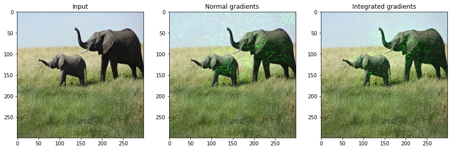
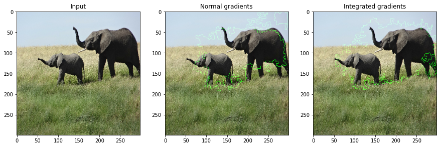
预测

# 1. Convert the image to numpy arrayimg = get_img_array(img_path)
# 2. Keep a copy of the original imageorig_img = np.copy(img[0]).astype(np.uint8)
# 3. Preprocess the imageimg_processed = tf.cast(xception.preprocess_input(img), dtype=tf.float32)
# 4. Get model predictionspreds = model.predict(img_processed)top_pred_idx = tf.argmax(preds[0])print("Predicted:", top_pred_idx, xception.decode_predictions(preds, top=1)[0])
# 5. Get the gradients of the last layer for the predicted labelgrads = get_gradients(img_processed, top_pred_idx=top_pred_idx)
# 6. Get the integrated gradientsigrads = random_baseline_integrated_gradients(np.copy(orig_img), top_pred_idx=top_pred_idx, num_steps=50, num_runs=2)
# 7. Process the gradients and plotvis = GradVisualizer()vis.visualize(image=orig_img,gradients=grads[0].numpy(),integrated_gradients=igrads.numpy(),clip_above_percentile=99,clip_below_percentile=0,)
vis.visualize(image=orig_img,gradients=grads[0].numpy(),integrated_gradients=igrads.numpy(),clip_above_percentile=95,clip_below_percentile=28,morphological_cleanup=True,outlines=True,)

专知，专业可信的人工智能知识分发，让认知协作更快更好！欢迎注册登录专知www.zhuanzhi.ai，获取5000+AI主题干货知识资料！

欢迎微信扫一扫加入专知人工智能知识星球群，获取最新AI专业干货知识教程资料和与专家交流咨询！

点击“阅读原文”，了解使用专知，查看获取5000+AI主题知识资源